How Does an Agent Learn? Teaching a Car to Drive

Series: Reinforcement Learning from scratch, with Agentic Racing as the lab

Part 1 · How Does an Agent Learn? Teaching a Car to Drive (this article)

Part 2 · How Do We Improve a Policy Without Breaking It? PPO Explained from Scratch

Part 3 · Can We Teach by Imitation? Behavioral Cloning Explained from Scratch

Part 4 · Can We Learn to Behave Like an Expert? GAIL Explained from Scratch

Part 5 · Can We Combine Imitation and RL? BC, GAIL, and PPO as One System

Introduction

When we think about teaching a person to drive, the answer seems fairly simple: we explain the rules, show examples, let them practice, and correct their mistakes.

But how do we do something similar with an artificial-intelligence agent?

At first, an agent doesn’t know what “turning”, “braking”, “going fast” or even “driving well” means. We can’t just tell it:

“Take this corner at 80 km/h.”

We have to build a world in which it can observe, act, receive a signal telling it whether its behavior was good or bad, and try again.

That is the starting point of Reinforcement Learning (RL).

In this article I’ll explain the fundamental ideas of RL using Agentic Racing, a racing simulation project built in Unity, as a hands-on lab. The goal isn’t to start with the math of a specific algorithm, but to first understand the problem we’re trying to solve.

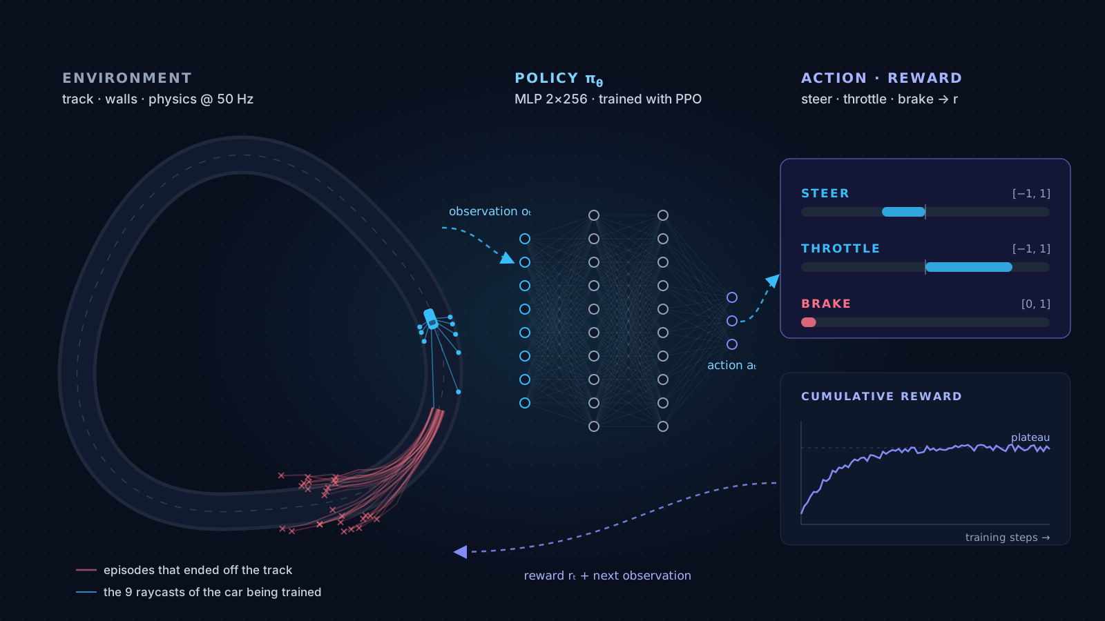
Before we start, an honest warning: in Agentic Racing the RL pilot never learned to complete a lap. Eight training runs with PPO plateaued at around 10–13% of a lap, and the demo ended up using a hand-written pilot. I told that story in detail in Agentic Racing: A Pilot That Never Learned to Drive. Far from making it a worse lab, that makes it a more useful one: every concept in this article has a real number behind it, a concrete design decision and, sometimes, a failure that explains it better than any textbook example.

The fundamental question is:

How does an agent learn what to do when nobody gives it the right answer directly?

1. Reinforcement learning as a game

The simplest way to picture Reinforcement Learning is as a repeated interaction between two elements:

an agent, which makes decisions;
an environment, which responds to those decisions.

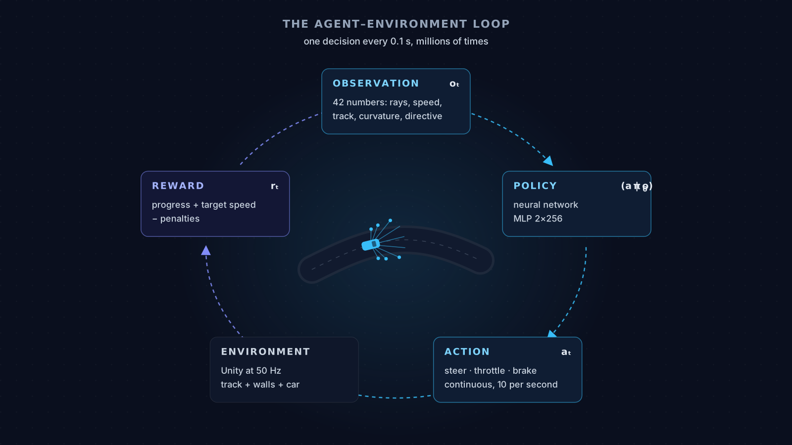
The agent–environment loop: the environment provides an observation, the policy chooses an action, the environment steps the physics and returns a reward together with the next observation.

The agent observes the environment, chooses an action, and receives the consequences of that action: a reward and a new observation.

Then it observes again and decides again.

And it repeats this process thousands or millions of times. In Agentic Racing, “millions” is literal: each training run was 4 to 20 million steps.

This matters because the agent does not receive the right answer at each step.

In supervised learning we might have:

input → correct answer

For example:

image of a corner → "turn left"

In Reinforcement Learning, instead, we have:

observation → action → consequence → reward

The agent has to discover which actions tend to produce better outcomes.

2. Our example: a car that wants to learn to drive

In Agentic Racing we have a very concrete problem:

We want a car to learn to drive inside a simulated racing environment.

That turns fairly abstract Reinforcement Learning concepts into something much easier to picture.

Our agent is inside a car. It has some information about what’s happening around it, it can control the steering, the throttle and the brake, and it receives signals telling it whether its behavior is helping or hurting its goal.

In the project, these pieces have names. The training environment is a TrainingArena: a circuit generated from a seed, with invisible walls along the edges. The agent is a RaceAgent, a class from ML-Agents (Unity’s RL toolkit). The actions are carried out by a CarController, which turns steering, throttle and brake into forces on a Rigidbody. And the physics is solved by the Unity engine 50 times per second:

                 ┌──────────────────────────────┐
                 │  TrainingArena               │
                 │  circuit (seed) + walls      │
                 └──────────────┬───────────────┘
                                │ observations (42 numbers)
                                ▼
                 ┌──────────────────────────────┐
                 │  RaceAgent (ML-Agents)       │
                 │  policy: MLP neural network  │
                 └──────────────┬───────────────┘
                                │ actions: steer, throttle, brake
                                ▼
                 ┌──────────────────────────────┐
                 │  CarController               │
                 │  forces on the Rigidbody     │
                 └──────────────┬───────────────┘
                                │
                                ▼
                 ┌──────────────────────────────┐
                 │  Unity physics (50 Hz)       │
                 │  position, velocity, heading │
                 └──────────────┬───────────────┘
                                │
                                ▼
                 ┌──────────────────────────────┐
                 │  TrackProgress               │
                 │  how far along the track?    │
                 └──────────────┬───────────────┘
                                │
                                ▼
                     reward + next observation

A practical detail: we don’t train with a single car. In the training runs, each scene contained 9 arenas, each with a circuit generated from a different seed, placed 4 km apart so that one car’s sensors can’t see the track next door. And we ran 4 processes of that scene in parallel. That made 36 cars feeding a single policy at the same time, driving nine different layouts so the policy wouldn’t just memorize one track.

And a bit of context: in the full design of the project, this pilot is only half of the system. Above it sits a “team boss”, an LLM that reasons about the race and radios down directives. In this article we stay with the pilot, which is where the RL lives.

3. What does “state” mean?

Before the agent can decide what to do, we need some way to describe the situation it’s in.

In Reinforcement Learning we usually talk about the state, which we write as:

s_t

where $t$ stands for the current time step.

Conceptually, the car’s state could contain information such as:

position relative to the track;
the car’s orientation;
speed;
how close the edges are;
the track geometry;
the direction of the next corner;
progress along the lap.

But here an important distinction appears.

State ≠ observation

The state $s_t$ ideally represents all the relevant information about the environment.

The agent, however, may not have direct access to all of that state. What it receives is an observation:

o_t

In other words:

“This is what the agent can see or know right now.”

A real self-driving system would have cameras, LiDAR, GPS, an IMU, speed, and so on. In a simulator we have the advantage of choosing what information we give the agent.

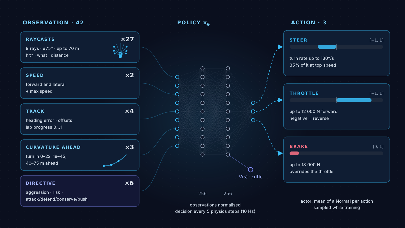
In Agentic Racing, the pilot receives 42 numbers at every decision:

Group	Count	What it contains
Raycasts	27	9 rays fanned out over ±75°, up to 70 m long, that detect the edge walls (3 values per ray: whether it hit, what it hit, and how far away)
Speed	2	forward and lateral speed, normalized by top speed
Relation to the track	4	heading error relative to the racing line, lateral offset of the car and of the racing line from the centerline, lap progress (0 to 1)
Curvature ahead	3	how much the track turns 0–22 m, 18–45 m and 40–75 m ahead
Directive	6	aggression, risk tolerance and the directive type (`attack`, `defend`, `conserve`, `push`)

Just as interesting is what it does not see: its absolute position on the map, the rest of the circuit beyond 75 meters, the other cars, the standings, or lap times. It’s a deliberately partial observation: that global context is exactly what the team boss sees, and the pilot doesn’t.

The last six numbers deserve an explanation. They are the channels through which the strategist talks to the pilot. During training nobody writes to them yet, so they are randomized every episode. That way the policy learns to drive differently depending on the directive it receives, instead of learning to ignore it. If you trained without those channels and added them later, you’d have to retrain from scratch.

This leads to a fundamental design decision.

If we give too much information, the problem can become artificially easy, or the policy can lean on data it won’t have when it’s used for real.

If we give too little, the agent may not have enough information to make good decisions.

Agentic Racing learned this the hard way. The first six runs didn’t have the three curvature-ahead observations. The agent could only “see” through the raycasts, which back then reached 40 m: at 15 m/s that’s less than three seconds of anticipation. It couldn’t see corners coming. The seventh run added curvature ahead and 70 m rays, together with a new speed reward. The critic started to understand the world much better (we’ll see that in section 9), but the fraction of the lap completed barely moved. A better observation was necessary, but not sufficient.

That’s why:

Designing the observations is also part of the Reinforcement Learning problem.

4. What can the agent do?

Now we need to define the actions. Let’s call an action:

a_t

In Agentic Racing, the action space is continuous and has three dimensions. The network doesn’t pick between options like “left” or “right”: it outputs three real numbers.

Action	Range	What it does in the `CarController`
`steer`	−1 to 1	turns the car at up to 130°/s, dropping to 35% of that at top speed
`throttle`	−1 to 1	applies up to 12,000 N of forward force; negative values mean reverse
`brake`	0 to 1	applies up to 18,000 N of braking and, while active, overrides the throttle (the network outputs values between −1 and 1; for the brake only the positive half counts)

On top of that there’s a lateral-grip model: when the car turns, the tires redirect most of the sideways velocity forward instead of losing it. We’ll see later why that detail mattered so much.

The agent doesn’t decide at every physics step. It decides every 5 steps, that is, 10 times per second, and repeats its last action between one decision and the next.

What happens inside the agent: 42 observations (raycasts, speed, relation to the track, curvature ahead and directive) feed a 2×256 MLP, which produces three continuous actions: steer, throttle and brake.

The agent might, for example, be facing a left-hand corner.

We don’t want to hand-code:

IF curve_is_left:
    steering = -0.42
    throttle = 0.71

We want the agent to learn a policy that figures out on its own which action makes sense given its observations.

5. The policy: the agent’s strategy

Here comes one of the most important concepts in all of RL.

The policy is the strategy the agent uses to choose actions.

Mathematically we can write:

\pi(a \mid s)

or, when we work explicitly with observations:

\pi(a \mid o)

The idea is:

“Given this situation, what should I do?”

In an agent based on a neural network, the policy is implemented as a parameterized function:

\pi_\theta

where $\theta$ stands for the parameters (the weights) of the neural network.

In our case, the network is a small MLP: 2 hidden layers of 256 neurons, with normalized observations. Because the actions are continuous, the network doesn’t output “the” action directly: it outputs the center of a normal distribution for each of the three actions. During training the action is sampled from that distribution, which lets the agent try variations. That’s why we write $\pi(a \mid o)$ as a probability rather than as a function that returns a single value.

At first, that policy doesn’t know how to drive. Its parameters don’t magically contain any racing knowledge.

We have to get them to change so that actions that lead to good outcomes become more and more likely.

And this is where the key element of reinforcement learning comes in.

6. The reward: telling the agent what we care about

How does the agent know an action was good?

We give it a reward. The reward at time $t$ is usually written as:

r_t

We can think of it as a numeric signal:

good action        → positive reward
bad action         → negative reward

But that’s a simplification. In a real RL problem, designing the reward is usually much harder.

This is what the RaceAgent reward function looked like in the last training run (the eighth), after seven versions:

Component	Type	Value	Why it exists
Progress	per meter	+0.02	moving forward along the track
Target speed	per second	up to +0.25	going at the right speed for the upcoming corner
Slowness	per second	up to ~−0.1	extra penalty only when far below that speed
Racing line	per second	up to +0.05	staying aligned with and close to the racing line, only while moving
Edge proximity	per second	up to −0.6	grows as the car gets closer to the wall
Wall hit	per event	−0.1	each contact with the edge
Stopped	per second	−0.3	while the car is stationary
Episode ended by failure	per event	−1	leaving the track, getting stuck, driving the wrong way, or not making progress
Lap completed	per event	+12, plus up to +8	finishing the lap, with a bigger bonus the faster it’s done

At each step, the reward is the sum of the components that apply:

r_t = r_{\text{progress}} + r_{\text{speed}} + r_{\text{line}} - r_{\text{edge}} - r_{\text{penalties}} + r_{\text{lap}}

The most interesting component is the speed one. In the early versions, more speed always meant more reward, so braking for a corner was pure cost, and the agent learned exactly that: never brake. The final version computes a target speed based on the upcoming curvature:

v_{\text{target}} = v_{\text{max}} \cdot \operatorname{lerp}\big(0.42,\ 0.12,\ \min(1,\ \theta / 55^\circ)\big)

where $\theta$ is the largest heading change of the track over the next ~55 meters. The reward peaks right at that speed and falls off on both sides:

r_{\text{speed}} = 0.25 \cdot \max\Big(0,\ 1 - 1.3\left|\frac{v - v_{\text{target}}}{v_{\text{target}}}\right|\Big) \cdot \Delta t

With that, braking before a tight corner stops being pure cost: there’s a zone where braking pays more than not braking.

7. The agent doesn’t learn from an isolated reward

Here comes one of the ideas that can feel counterintuitive at first.

Suppose the car does this:

accelerates
   ↓
approaches a corner
   ↓
brakes
   ↓
turns
   ↓
stays on the track
   ↓
makes a lot of progress

The important reward doesn’t show up right after braking. In fact, at the moment it brakes, the car moves forward less and earns less progress reward. The benefit arrives seconds later, when it stays on the track instead of crashing.

That’s why we don’t want the agent to simply ask:

“Did this action give me a reward?”

We want it to learn:

“What future consequences did my actions have?”

That brings us to the concept of return.

8. Return: thinking about future rewards

The return is the accumulated reward we get from a given moment onward.

A common formulation is:

G_t = r_t + \gamma r_{t+1} + \gamma^2 r_{t+2} + \gamma^3 r_{t+3} + \dots = \sum_{k=0}^{\infty} \gamma^k r_{t+k}

where:

0 \leq \gamma \leq 1

is the discount factor.

The parameter $\gamma$ controls how much we value future rewards. If $\gamma$ is close to 1, the agent takes more distant consequences into account. If it’s smaller, it pays relatively more attention to immediate rewards.

We can picture it like this:

now            near future          far future

 rₜ       +      γ rₜ₊₁       +       γ² rₜ₊₂
 │                 │                    │
weight 1        weight γ            weight γ²

In Agentic Racing we use $\gamma = 0.995$ , and the discount is applied per decision, that is, every 0.1 seconds. That gives a very concrete sense of how far “ahead” the agent looks:

a reward 200 decisions away (20 seconds) is weighted by $0.995^{200} \approx 0.37$ ;
a reward 900 decisions away (90 seconds, roughly the length of a lap) is weighted by $0.995^{900} \approx 0.01$ .

In other words, the braking that saves a corner two seconds from now is well within the agent’s horizon. The bonus for finishing the lap, seen from the start, barely exists. That’s why the reward needs dense signals, like progress or target speed, that arrive early.

All of this lets us express something very important:

An action can be bad in the short term but good in the long term.

Braking before a corner momentarily reduces speed, but it lets you take the corner better and finish the lap faster. The agent has to learn that kind of relationship.

9. How do we know whether a state is good?

Here comes another fundamental concept: the value function.

V^\pi(s) = \mathbb{E}_\pi\left[\, G_t \mid s_t = s \,\right]

The value function tries to estimate:

“If I’m in this state and keep following this policy, how much future reward do I expect to get?”

                    state
                      │
                      ▼
              ┌──────────────┐
              │     V(s)     │
              └──────┬───────┘
                     │
                     ▼
               expected value

A state like:

car centered
+ good speed
+ entering a corner
  correctly

might have a high value. Whereas:

car pinned against the wall
+ wrong orientation
+ low speed

might have a low value.

The value function doesn’t tell you directly which action to take. It says something closer to:

“How promising is this situation?”

In PPO, this function is learned by a second network, known as the critic, which is trained alongside the policy. ML-Agents reports how well it predicts through a metric called Value Loss. In the early Agentic Racing runs that loss went up over training (from 0.12 to 0.27 in the first run, and up to 0.52 in the sixth): the critic couldn’t anticipate what was about to happen. Once the agent started receiving the track curvature ahead, the loss stayed stable at 0.22. With better observations (and a new reward in the same run), the critic could finally tell a promising state from a doomed one. A critic that understands the world, however, doesn’t guarantee that the policy learns to move well in it.

10. Q(s,a): valuing a specific action

We can also ask a slightly different question:

“How good is this specific action in this state?”

That leads us to:

Q^\pi(s,a) = \mathbb{E}_\pi\left[\, G_t \mid s_t = s,\ a_t = a \,\right]

The conceptual difference is:

V(s)
│
└── How good is it to be here?

Q(s,a)
│
└── How good is it to take this action here?

For example:

State:
tight left-hand corner, at high speed

Action A:
keep accelerating

Action B:
brake and turn

Q(s,A) → probably lower
Q(s,B) → probably higher

We don’t know the exact values in advance. The agent has to estimate them from its experience.

11. Advantage: was this action better than expected?

Now we can combine the previous ideas.

The advantage is defined as:

A^\pi(s,a) = Q^\pi(s,a) - V^\pi(s)

The interpretation is extremely useful:

“Is this action better or worse than what I usually expect in this state?”

If $A(s,a) > 0$ , the action is better than the average of what the policy usually does there.

If $A(s,a) < 0$ , it’s worse.

In practice we don’t know $Q$ or $V$ exactly. The advantage is estimated from the rewards observed after each action and from the critic’s prediction. That’s the role of the lambd: 0.95 parameter in our configuration, which we’ll cover in the next article.

This is especially important for algorithms like PPO, which we’ll look at in the next article.

12. So how does the network actually learn?

So far we have:

observation
     ↓
policy
     ↓
action
     ↓
environment
     ↓
reward
     ↓
experience

The learning process consists of using those experiences to modify the policy’s parameters.

At first we have a practically useless policy:

observation
    ↓
"turn"
    ↓
leaves the track

After many experiences, we want the actions that have historically produced better outcomes to become more likely.

In ML-Agents, that cycle has concrete numbers. The 36 cars collect experience until they fill a buffer of 20,480 decisions. With that buffer, the network makes 3 passes in batches of 2,048. Then the experience is thrown away and new experience is collected with the updated policy. PPO is an on-policy algorithm: it only learns from experience generated by its current version.

                 EXPERIENCE

      ┌───────────────────────────────┐
      │ observation                   │
      │ action                        │
      │ reward                        │
      │ next observation              │
      └───────────────┬───────────────┘
                      │
                      ▼
                  learning
                      │
                      ▼
                update policy
                      │
                      ▼
                 new policy
                      │
                      ▼
               more experience
                      │
                      └───────────► ...

The agent enters a loop:

observe → act → receive feedback → learn → act again

13. Training is different from execution

There’s another important distinction.

During training we want the agent to explore. When running a trained policy, we want it to make useful decisions.

              TRAINING

      explore → make mistakes
          ↓
      receive reward
          ↓
      update policy
          ↓
      try again

Exploration in Agentic Racing comes from two places: actions are sampled from a distribution (the most likely one isn’t always taken), and the algorithm rewards that distribution for not narrowing too early, through an entropy term (the beta parameter in the configuration). The policy’s entropy is a good measure of how much it’s exploring. In the first run it dropped from 1.42 to 0.82 over 20 million steps: the agent became more and more sure of itself, although, as we’ll see, not necessarily about the right things.

Once trained, the policy is exported to an .onnx file and runs without the training algorithm. The plan was to run it inside the browser with Unity’s inference engine. That part was validated in the project with a toy model, at 0.1 ms per inference. The problem was elsewhere.

The goal of training isn’t to avoid every mistake. Mistakes are precisely a source of information. If the car turns too early and leaves the track, that experience helps the policy learn that the behavior is undesirable.

Of course, for this to work we need:

a reasonably correct environment;
informative observations;
well-defined actions;
a suitable reward function;
an appropriate learning algorithm.

And here an important engineering lesson appears:

If the agent doesn’t learn, that doesn’t necessarily mean the RL algorithm is wrong.

The problem can be in any piece of the system.

14. The environment is part of the problem too

This point is especially important in Agentic Racing.

An RL algorithm can be mathematically correct and still produce an agent that doesn’t learn. Why? Because the agent learns from the world we built for it.

                    ┌──────────────┐
                    │ OBSERVATIONS │
                    └──────┬───────┘
                           │
                           ▼
                    ┌──────────────┐
                    │    POLICY    │
                    └──────┬───────┘
                           │
                           ▼
                    ┌──────────────┐
                    │    ACTIONS   │
                    └──────┬───────┘
                           │
                           ▼
              ┌────────────────────────┐
              │      ENVIRONMENT       │
              │                        │
              │ physics + track + car  │
              └────────────┬───────────┘
                           │
                           ▼
                         REWARD
                           │
                           └──────► LEARNING

Every block can become a source of problems, and in Agentic Racing almost all of them did:

If the reward is badly designed, the agent finds a way to maximize it without doing the task. This is known as reward hacking. In the fourth run, stopping ended the episode with a −1 penalty. The agent learned the optimal policy for that reward: use the rolling start, roll about 245 meters collecting progress ( $245 \times 0.02 = 4.9$ ), stop, and accept the −1. That came out to about +4 per episode, very close to where the training curve plateaued. Dying quickly was the best strategy available. The fix was for stopping to no longer end the episode and to cost something for every second instead.

If the reward pushes in the wrong direction, same thing. Rewarding the agent for following the racing line seemed reasonable, but in this project the racing line runs right along the edges in every corner. Rewarding it pushed the car into the walls.

If the physics behaves unexpectedly, the agent learns strange strategies. The original lateral-grip model erased the car’s sideways velocity instead of redirecting it. The result: turning hard at 13 m/s brought the car almost to a dead stop. Any aggressive turn was a sudden brake, so both the agent and the reference controller “learned” not to turn, which is the same as not taking corners.

If the world is broken, nothing makes up for it. The procedurally generated tracks had sections with degenerate geometry and corners that not even a hand-written controller could take.

That’s why an RL project isn’t simply:

install PPO
↓
train
↓
get a self-driving car

15. The RL pilot’s spec sheet

With all the pieces on the table, this is how the problem was defined across the eight training runs:

Piece	In Agentic Racing
Framework	Unity ML-Agents 4.0.3 (Unity package) and `mlagents` 1.1.0 (Python)
Algorithm	PPO
Observation	42 numbers: 27 from raycasts, plus 15 for speed, relation to the track, curvature ahead and directive
Actions	3 continuous: `steer` and `throttle` in [−1, 1], `brake` in [0, 1]
Frequency	physics at 50 Hz, one decision every 5 steps (10 per second)
Network	MLP with 2 layers × 256 neurons, normalized observations
Hyperparameters	$\gamma = 0.995$ , $\lambda = 0.95$ ; learning rate $3 \times 10^{-4}$ , $\epsilon = 0.2$ and `beta` = 0.01 (0.005 in the first run) as initial values, with linear decay
Episode	one lap; the car spawns at a random point on the circuit, with heading noise (±10°) and position noise (±2 m), already rolling at 8 m/s
Episode end	lap completed; more than 2 m off the track; 8 s stopped; 4.5 s going the wrong way; less than 8 m of progress in 5 s; or 4,000 physics steps (~80 s)
Progress	meters advanced along the circuit’s centerline, measured every step
Parallelism	9 arenas per process × 4 processes = 36 cars, on 9 different procedural circuits

(The code has changed since then: today the arenas use a single fixed circuit and the limit is 6,000 steps, because a lap of that circuit takes about 95 seconds.)

And here’s how it went. Eight runs, 4 to 20 million steps each, with seven versions of the reward and several physics fixes. The fraction of the lap the car completed before the episode ended always stayed around 10% (between 8 and 13%). In the eighth run, 91% of episodes ended with the car off the track.

To separate learning problems from environment problems, the project used a hand-written controller, with no learning at all, on the same physics and the same tracks. Its best episode reached 82% of a lap at 21 m/s, but on average it got stuck almost as often as the RL agent. That already said something: if a hand-designed controller couldn’t handle those tracks either, the problem wasn’t just learning. The confirmation came from switching to a fixed, clean circuit, with no procedural generation. There, that controller completed full laps without a single incident.

16. What happens at the beginning?

Let’s imagine we start training with a policy that doesn’t know how to drive yet.

The initial behavior is essentially chaotic:

      🏎️
       \
        \
         → off the track

In Agentic Racing’s first run, during the first 50,000 steps, episodes lasted about four seconds and the mean reward was negative (−1.1). The car barely got going before leaving the track or stopping.

The agent has no human representation of:

“This is a dangerous corner.”

All it has is numbers. It doesn’t think:

“I’m going too fast.”

It has an observation containing certain values, and it has to learn the relationship between those values, the actions, and the consequences.

After enough experience, we want patterns like this one to emerge:

observation:
tight corner + high speed
            │
            ▼
         brake
            │
            ▼
      turn better
            │
            ▼
     stay on track
            │
            ▼
      more reward

And those patterns end up encoded in the policy’s parameters.

In Agentic Racing, that particular pattern never emerged. When the policies from the third and fourth runs were evaluated, the average brake value was 0.02 out of 1: the agent practically never braked. It had learned one of two things. Either it crawled at 7 m/s so it could turn without braking, or it went full throttle and ended up off the track or stopped shortly after the first real corner.

Why didn’t it figure it out? In the seventh run, with a reward that already paid for braking before corners, the hypothesis was a hard-exploration problem. The full corner maneuver (brake, turn, accelerate again) is a coordinated sequence lasting one or two seconds. 97% of episodes ended off the track about 200 meters from the start, right at that first corner. The agent reached the corner over and over, but almost never stumbled onto the right sequence by chance, so it almost never had the experience that would have taught it that braking was worth it.

That hypothesis was only partly right. Later on, the physics and track-geometry problems from section 14 surfaced, and they made that maneuver much harder than it should have been.

17. Are we programming the driving rules?

Not exactly. This is a fundamental difference between a traditional controller and a learned agent.

In a rule-based system we would write something like this, which is a simplified version of the reference controller that exists in the project:

corner_ahead = largest heading change over the next 60 m
target_speed = lerp(40% of vmax, 10% of vmax, corner_ahead / 45°)

IF speed < target_speed:
    accelerate
ELSE IF speed > target_speed + margin:
    brake
steering = aim at a point on the racing line, 12 to 36 m ahead

In Reinforcement Learning we try to make the behavior emerge from the learning process. We define:

what the agent can observe;
what actions it can take;
what consequences each action has;
what rewards it receives;
which algorithm it will use to learn.

But we don’t hand-specify the driving decisions.

That’s exactly what makes it interesting, and also what makes it hard. The rule-based controller above is the one that drives the cars in the demo today. The directive channels the RL agent had in its observations now modulate those rules directly: more aggression means a higher target speed and braking later. To demonstrate the relationship between pilot and strategist, a hand-written pilot whose behavior changes with the directive met the requirement. Getting to the same point with RL would have taken more iterations than the project could afford. On the fixed circuit, where the track is no longer an obstacle, PPO would probably learn to complete laps, but that experiment is still pending.

18. From individual behavior to a policy

After enough interactions, the neural network tries to approximate a function:

\pi_\theta(a \mid o)

That is:

“Given this observation, which action should I produce?”

The network doesn’t store an explicit list of rules. Instead of:

if curve then brake
if straight then accelerate
if left then steer left

it learns a continuous, parameterized function:

                    OBSERVATION (42)
                         │
                         ▼
                ┌─────────────────┐
                │                 │
                │  MLP 2 × 256    │
                │                 │
                └────────┬────────┘
                         │
             ┌───────────┼───────────┐
             ▼           ▼           ▼
         steering     throttle      brake

The challenge is getting that function to improve in a stable way.

And that’s where our next algorithm comes in.

19. The next step: PPO

Up to this point we’ve built the conceptual map:

Agent
  │
  ├── observes
  │
  ├── chooses an action
  │
  ├── receives reward
  │
  ├── accumulates experience
  │
  ├── estimates which states/actions are good
  │
  └── improves its policy

But we still haven’t explained how we update the policy mathematically.

One of the best-known answers is Proximal Policy Optimization (PPO), the algorithm Agentic Racing used in all of its runs.

PPO introduces an especially interesting idea:

We want to improve the policy, but we don’t want to change it too much from one update to the next.

Why? Because an overly aggressive update could destroy behaviors that were already working.

The intuition is:

Current policy
     │
     │ small improvement
     ▼
New policy
     │
     │ small improvement
     ▼
New policy
     │
     ▼
...

instead of:

Current policy
     │
     │ big jump
     ▼
Completely different policy
     │
     ▼
unstable behavior

PPO compares the probability that the new and the old policy assign to each action, weights it by the advantage, and stops rewarding changes that move too far. The epsilon: 0.2 in our configuration sets that limit: once the ratio between an action’s new and old probability moves more than 20% away from 1, moving it further no longer improves the objective.

The mathematical detail of this mechanism will be the topic of the next article.

20. But Agentic Racing taught us something even more important

When we build a real RL system, the algorithm is just one piece. Changing any of the others (what the agent sees, what it can do, what it’s rewarded for, the physics it experiences) can completely change the learned behavior.

That’s why, when an agent doesn’t learn, the question shouldn’t only be:

“Which PPO parameter do I need to change?”

We should also ask:

“What is the agent seeing?”

“What can it do?”

“What reward is it receiving?”

“What physical dynamics is it experiencing?”

“Is the environment providing a coherent learning signal?”

In Agentic Racing, all five questions had uncomfortable answers at some point: it couldn’t see corners coming, the reward had an easy way out, the physics turned every turn into a sudden brake, and the track itself had impossible sections. None of those problems could be fixed by touching PPO’s hyperparameters. Every run used PPO; what changed from one to the next was the reward, the agent’s perception, or the physics.

The lesson that stuck with me most: before spending compute on a sophisticated method, validate that the environment can be solved with a simple one. If a hand-written controller can’t complete a lap, it’s unlikely that a reward will teach a neural network to do it.

21. The complete mental map

We can summarize everything so far like this:

                       AGENT
                         │ observes
                         ▼
                    OBSERVATION
                         │
                         ▼
                      POLICY
                         │ chooses
                         ▼
                      ACTION
                         │
                         ▼
                    ENVIRONMENT
                         │
             ┌───────────┴───────────┐
             ▼                       ▼
        NEW STATE                 REWARD
             └───────────┬───────────┘
                         ▼
                    EXPERIENCE
                         │
                         ▼
                 LEARNING ALGORITHM
                         │
                         ▼
                  UPDATED POLICY ──────► ...

The mathematical concepts we’ll keep building form a chain:

\begin{gathered} \text{Observation} \rightarrow \text{Action} \rightarrow \text{Reward} \rightarrow \text{Return} \\ \rightarrow V \rightarrow Q \rightarrow \text{Advantage} \rightarrow \text{Policy learning} \end{gathered}

We don’t need to memorize all of these formulas yet. What matters is understanding which question each one answers:

Concept	Question
Observation	What can the agent see?
Action	What can it do?
Reward	How good was the immediate consequence?
Return	How much accumulated reward do I get from here?
Value $V(s)$	How promising is this situation?
Q-value $Q(s,a)$	How good is this action in this situation?
Advantage $A(s,a)$	Is this action better or worse than expected?
Policy $\pi(a \mid s)$	Which action should I choose?

With this map we can start studying algorithms like PPO without treating them as a collection of disconnected formulas.

22. One last idea: the agent learns from experience, not from explanations

This may be the most important idea to take away from this article.

We can look at a corner and say:

“You need to brake here.”

The agent doesn’t get that explanation. It gets data, acts, observes the consequences, gets a reward, and repeats.

Millions of small interactions can turn an initially useless policy into one that produces complex behavior.

That’s what’s fascinating about Reinforcement Learning:

We don’t program the final behavior directly. We design a process through which the agent can discover it.

And Agentic Racing shows the other side of that sentence: if the process is badly designed, the agent discovers something else. It discovered that stopping paid more than continuing, that turning was dangerous, and that braking was pointless. Each of those lessons was perfectly rational given the world and the reward we gave it. The agent learned what we taught it, which wasn’t what we meant to teach it.

In the next article we’ll open up the PPO box: what exactly it does with all that experience, and why its way of updating the policy is so stable.

What’s next

Next article in the series (part 2):

How Do We Improve a Policy Without Breaking It? PPO Explained from Scratch

In it we build, step by step:

Policy Gradient
Actor-Critic
Value Function
Advantage
GAE
Probability Ratio
Clipping
PPO Objective
The full training loop
How all of this shows up in Agentic Racing

And above all, we answer one question:

Why does PPO work better when we stop it from changing its mind too quickly?

The agent code (RaceAgent.cs), the training configuration (race_ppo.yaml) and the full log of all eight runs are at github.com/alulema/agentic-racing.