How Do We Improve a Policy Without Breaking It? PPO Explained from Scratch

Series: Reinforcement Learning from scratch, with Agentic Racing as the lab

Part 1 · How Does an Agent Learn? Teaching a Car to Drive

Part 2 · How Do We Improve a Policy Without Breaking It? PPO Explained from Scratch (this article)

Part 3 · Can We Teach by Imitation? Behavioral Cloning Explained from Scratch

Part 4 · Can We Learn to Behave Like an Expert? GAIL Explained from Scratch

Part 5 · Can We Combine Imitation and RL? BC, GAIL, and PPO as One System

Where we left off

Part 1 ended with a conceptual map: the agent observes, chooses an action, receives a reward, accumulates experience, and estimates which states and actions are good. What was missing was the last arrow: how that experience is used to improve the policy.

And it ended with a question:

Why does PPO work better when we stop it from changing its mind too quickly?

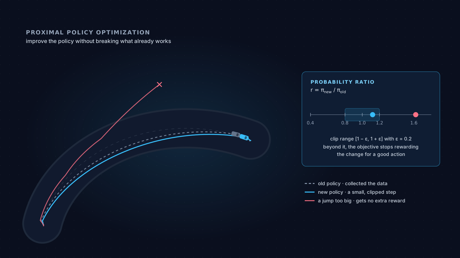
This article answers that question. Picture a virtual driver that has already learned something useful (staying on track on the straights, taking a gentle corner) but still makes mistakes. We want it to improve without a training update destroying what already works.

Proximal Policy Optimization (PPO) is an algorithm that updates the policy (the strategy that decides which action to take) while controlling how much it changes on each update. Proximal means close: the new policy shouldn’t drift too far from the one that generated the experience it’s learning from.

As in part 1, every idea comes with what the Unity ML-Agents trainer actually does (version 1.1.0 of the Python package) and how it was configured in Agentic Racing. And, as in part 1, with an honest warning: in this project the RL pilot never learned to complete laps consistently. That doesn’t make the example less useful. Seeing what PPO optimized when it didn’t learn what we wanted is one of the best ways to understand what it optimizes.

1. A thirty-second recap

From part 1 we need three pieces.

The policy is a parameterized function that assigns probabilities to actions:

\pi_\theta(a \mid s)

where $s$ is the state (in practice, the agent’s observation), $a$ is an action, and $\theta$ are the neural network’s weights. In Agentic Racing, $s$ is 42 numbers (raycasts, speed, relation to the track, curvature ahead and the strategist’s directive) and $a$ is three continuous actions: steer, throttle and brake. Because the actions are continuous, the network outputs the center of a normal distribution for each one, and the action is sampled from that distribution.

The advantage compares an action with what’s normally expected in that state:

A(s,a) = Q(s,a) - V(s)

$A(s,a) > 0$ : the action was better than expected.
$A(s,a) < 0$ : it was worse than expected.
$A(s,a) \approx 0$ : it was close to what was expected.

And the critic is the part of the system that estimates $V(s)$ , the expected return from a state.

That’s enough.

2. Policy gradient: nudging probabilities in the right direction

The most direct idea for improving a policy is this: raise the probability of actions that turned out better than expected, and lower it for those that turned out worse. That’s what policy gradient methods do. Their best-known form estimates the gradient of performance like this:

\nabla_\theta J(\theta) \approx \mathbb{E}_t\left[\nabla_\theta \log \pi_\theta(a_t \mid s_t)\, \hat{A}_t\right]

You don’t need to follow the derivation to get the intuition:

$\nabla_\theta \log \pi_\theta(a_t \mid s_t)$ tells us which way to move the weights to make action $a_t$ more likely in state $s_t$ .
$\hat{A}_t$ (the hat means it’s an estimate) sets the direction and size of the nudge: if the action turned out better than expected, we make it more likely; if worse, less.

This works, but it has two practical problems.

The first: step size. $\hat{A}_t$ is a noisy estimate. If we take too large a step along the gradient, the policy can change so much that it starts doing things it has never tried and for which our estimates say nothing. One bad step can undo in a single update what took millions of steps to learn.

The second: experience is expensive. In Agentic Racing, each update needs 20,480 decisions. At 10 decisions per second, that’s about 34 minutes of simulated driving, spread across the 36 cars training in parallel. Using that experience for a single gradient step and throwing it away would be a waste. We want to reuse it several times.

But as soon as we take the first gradient step, the policy is no longer the one that collected that experience. We need a way to measure how far it has moved. That’s where the probability ratio comes in.

3. The probability ratio: how much did the policy change?

PPO compares the policy we’re optimizing with the one that collected the experience:

r_t(\theta) = \frac{\pi_\theta(a_t \mid s_t)}{\pi_{\theta_{\text{old}}}(a_t \mid s_t)}

$r_t = 1$ : the probability of that action didn’t change.
$r_t = 1.2$ : the new policy gives that action a 20% higher probability.
$r_t = 0.8$ : the probability is 20% lower.

With continuous actions, as in our car, probability densities are compared instead of probabilities, but the idea is the same. ML-Agents computes it from logarithms, which is numerically more stable: r_theta = torch.exp(log_probs - old_log_probs).

One detail worth keeping in mind: this ratio compares action probabilities. It does not mean the car got 20% better in speed, safety, or lap time.

With this ratio, the policy-gradient objective can be rewritten as $r_t(\theta)\,\hat{A}_t$ . At the start of the update $r_t = 1$ and the gradients of both forms match. As the policy changes, $r_t$ corrects for the fact that we’re evaluating actions chosen by an older policy. It only corrects the actions, not the states: the situations the car ended up in are still the ones the old policy produced. That’s another reason not to drift too far. That lets us reuse the same batch of experience over several passes.

But it also opens the door to the step-size problem: if we maximize $r_t\,\hat{A}_t$ without limits, the optimizer will want to push $r_t$ up endlessly for every action with a positive advantage. We need a brake.

4. Clipping: removing the incentive to change too much

PPO’s clipped objective is:

L^{\text{CLIP}}(\theta) = \mathbb{E}_t\left[\min\Big(r_t(\theta)\,\hat{A}_t,\ \operatorname{clip}\big(r_t(\theta),\, 1-\epsilon,\, 1+\epsilon\big)\,\hat{A}_t\Big)\right]

It has three parts:

$r_t(\theta)$ measures how much an action’s probability changed.
$\hat{A}_t$ estimates whether that action was better or worse than expected.
clip cuts the ratio to the interval $[1-\epsilon,\, 1+\epsilon]$ in one of the two terms, and the min keeps the more pessimistic of the two.

In Agentic Racing, $\epsilon$ started at 0.2, so the interval was:

[1-\epsilon,\ 1+\epsilon] = [0.8,\ 1.2]

The clearest way to understand it is to look at the four possible cases:

Case	Example	Which term does the `min` pick?	Effect
Good action ( $\hat{A} > 0$ ) that already went up a lot	$r_t = 1.5$	the clipped one: $1.2\,\hat{A}$	the objective stops growing; no more incentive to raise it
Good action ( $\hat{A} > 0$ ) that went down	$r_t = 0.5$	the unclipped one: $0.5\,\hat{A}$	the gradient keeps pushing to raise it again
Bad action ( $\hat{A} < 0$ ) that already went down a lot	$r_t = 0.5$	the clipped one: $0.8\,\hat{A}$	the objective stops improving; no more incentive to lower it
Bad action ( $\hat{A} < 0$ ) that went up	$r_t = 1.5$	the unclipped one: $1.5\,\hat{A}$	the gradient keeps pushing to lower it

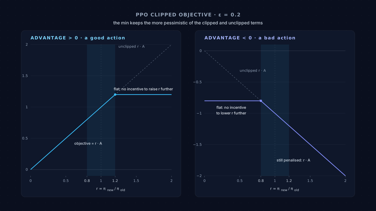
PPO's clipped objective as a function of the ratio r. With a positive advantage, the objective grows with r up to 1.2 and then goes flat. With a negative advantage, the objective improves as r drops to 0.8 and below that point goes flat. Outside those flat zones, the objective follows the unclipped line.

The pattern is asymmetric on purpose. PPO stops rewarding changes that go too far in the “good” direction, but it doesn’t stop penalizing changes that go the wrong way. It’s a pessimistic bound: the objective is never more optimistic than the unclipped version.

And this is the answer to the question part 1 ended with. PPO works better when we stop it from changing its mind too quickly because advantage estimates are only reliable close to the policy that generated the data. If the policy drifts far away, it starts making decisions in situations nobody measured, with advantages computed for a different policy. Clipping keeps each update in the zone where the data still says something true. That’s what lets the batch be reused several times without a noisy estimate dragging the policy away from what already worked.

An important nuance: clipping doesn’t forbid $r_t$ from leaving the $[0.8,\ 1.2]$ interval. It removes the benefit the objective assigns to certain extreme changes, depending on the sign of the advantage, but the ratio can still go past that limit during an update. It’s a practical optimization mechanism, not an absolute guarantee that every update is small.

In ML-Agents, the implementation follows the equation very closely (the loss is minimized, hence the minus sign):

r_theta = torch.exp(log_probs - old_log_probs)
p_opt_a = r_theta * advantage
p_opt_b = torch.clamp(r_theta, 1.0 - epsilon, 1.0 + epsilon) * advantage
policy_loss = -1 * masked_mean(torch.min(p_opt_a, p_opt_b), loss_masks)

One detail the equation doesn’t show: with continuous actions, ML-Agents computes and clips one ratio per action dimension. In our car that’s three ratios (steer, throttle and brake), each with its own clip, which are then averaged, instead of a single ratio for the joint action.

5. Actor-critic: one network decides, the other estimates

Common PPO implementations use an actor-critic setup:

The actor is the policy: it receives the observation and decides which action to take.
The critic estimates $V(s)$ , the expected return from the current state.

The critic is what lets us compute whether experiences turned out better or worse than expected. It isn’t infallible: if its estimates are off, the advantages will be too, and the actor will learn from the wrong signals.

In ML-Agents, with the default configuration, the actor and the critic are two separate networks with the same shape. In Agentic Racing they were two MLPs with 2 layers of 256 neurons each. Both are trained together, with a single loss function:

L = L^{\text{policy}} + 0.5\, L^{\text{value}} - \beta\, H(\pi_\theta)

$L^{\text{policy}}$ is the clipped objective from the previous section, with the sign flipped.
$L^{\text{value}}$ is the critic’s error when predicting the return. In ML-Agents it’s also clipped with the same $\epsilon$ : if the new prediction moves more than $\epsilon$ away from the old one, the error is computed with the more pessimistic version, so moving further doesn’t reduce the loss.
$H(\pi_\theta)$ is the policy’s entropy, and $\beta$ its weight. Subtracting it rewards the policy for not becoming too sure of itself too soon, so it keeps exploring. In Agentic Racing, $\beta$ was 0.005 in the first run and 0.01 from the second onward, always as the initial value.

Part 1 showed this critic in action. In the first runs, its error (ML-Agents’ Value Loss metric) went up over training: it couldn’t anticipate what was about to happen. In the seventh run, when the agent started seeing the track curvature ahead, it stayed stable at 0.22, although that same run also changed the speed reward.

6. TD error and GAE: estimating the advantage

One question remains: where does $\hat{A}_t$ come from?

A common signal is the temporal-difference error (TD error):

\delta_t = r_t + \gamma\, V(s_{t+1}) - V(s_t)

Here $r_t$ is the reward (not to be confused with the ratio $r_t(\theta)$ from section 3; standard notation uses the same letter for both), $\gamma$ is the discount factor, and $V$ are the critic’s estimates. $\delta_t$ answers a concrete question: “after this action, did things turn out better or worse than the critic expected?”.

A single $\delta_t$ only looks one step ahead. Summing many looks further but accumulates more noise. PPO usually uses Generalized Advantage Estimation (GAE), which combines both extremes:

\hat{A}_t^{\text{GAE}(\gamma,\lambda)} = \sum_{l=0}^{\infty} (\gamma\lambda)^l\, \delta_{t+l}

$\gamma$ controls the weight of future rewards and $\lambda$ how TD errors are combined over time. With $\lambda = 0$ only the immediate step counts (little noise, but heavily dependent on the critic being right). With $\lambda = 1$ everything that happened afterward counts (less dependence on the critic, but much more noise).

In Agentic Racing, $\gamma = 0.995$ and $\lambda = 0.95$ , so the factor in the sum is $\gamma\lambda \approx 0.945$ . That has a concrete reading:

a TD error’s weight halves every ~12 decisions, that is, every ~1.2 seconds;
most of an action’s advantage is decided by what happens in the next two or three seconds.

It’s interesting to compare this with part 1, where we saw that the return looks about 20 seconds ahead. Both are compatible: GAE looks only a short way ahead explicitly, but every $\delta$ includes $V(s_{t+1})$ , and the critic’s estimate already summarizes the more distant future. That’s why a critic that doesn’t understand the world ruins the advantages, however well designed everything else is.

In practice, ML-Agents computes the sum over the available experience. When a trajectory is cut off before the episode ends (for example, when it hits the step limit), it uses the critic’s estimate of the last state so it doesn’t pretend the future is worth zero. And before optimizing, it normalizes the advantages in the batch (mean 0, standard deviation 1), so what matters is which actions did better than the others in that same batch, not the absolute value.

7. The PPO training loop

With all the pieces, the full loop looks like this:

Use the current policy to interact with the environment.
Collect trajectories: observations, actions, rewards, and the probabilities the policy assigned to them.
Estimate values with the critic and advantages with GAE.
Optimize for several epochs over the batch, in minibatches.
In each minibatch, compute the ratio between the new policy and the old one.
Apply the clipped objective.
Update actor and critic with the combined loss.
Discard the batch and repeat with fresh experience.

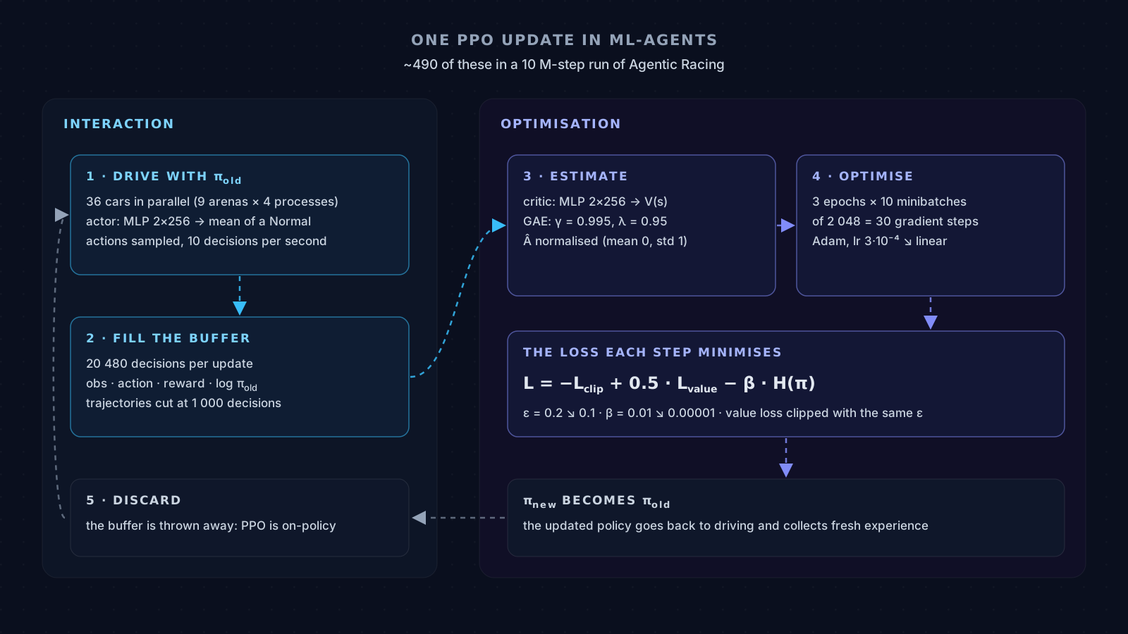
PPO's loop in ML-Agents with Agentic Racing's numbers: 36 cars collect experience until a buffer of 20,480 decisions is full; the critic estimates V(s) and GAE computes the advantages, which are normalized; over 3 epochs, 10 minibatches of 2,048 update actor and critic with the clipped objective; then the buffer is discarded and the new policy goes back to driving.

PPO is an on-policy method: it learns from experience generated by its current version or a very recent one. It can reuse the batch for a few epochs (that’s what the ratio and clipping are for), but it isn’t designed to reuse any historical experience indefinitely, the way off-policy methods do.

In Agentic Racing, the loop had these numbers:

Step	Value in `race_ppo.yaml`	What it means
Collection	`buffer_size: 20480`	each update uses 20,480 decisions, gathered by 36 cars
Optimization	`num_epoch: 3`, `batch_size: 2048`	3 passes over the batch, in 10 minibatches: 30 gradient steps per update
Clipping	`epsilon: 0.2`, `linear`	starts at 0.2 and decays linearly to 0.1 by the end of training
Learning rate	`learning_rate: 3.0e-4`, `linear`	decays linearly to almost zero
Entropy	`beta: 1.0e-2`, `linear`	decays linearly to 0.00001
GAE	`gamma: 0.995`, `lambd: 0.95`	the horizon from the previous section
Trajectories	`time_horizon: 1000`	cut every 1,000 decisions at most; since episodes lasted at most 800, in practice the critic only filled in the rest when time ran out
Length	`max_steps: 10000000`	a little under 490 policy updates in a 10-million-step run

The three linear schedules do the same thing on different knobs: early in training the policy can change more and explore more; by the end, changes get smaller and smaller. It’s another way of “not changing its mind too quickly”, this time over the whole run.

8. What PPO did in Agentic Racing

Let’s go back to part 1’s story with these pieces in hand. Eight runs, 4 to 20 million steps each, and the mean lap fraction always stayed around 10% (between 8 and 13%). Did PPO fail?

Not exactly. The training curves show that PPO did its job: it optimized, stably, exactly the objective we gave it.

It converged, and quickly. In the first run, mean reward went from −1.1 to 3.35 in the first ~1.85 million steps and then stayed flat for the remaining 18 million. In the eighth, reward was flat from ~2.7 million steps on. The pattern repeated in almost every run: a stable climb and a plateau. The exception was the third, which didn’t flatten out within its 4 million steps; with more training, the fourth went back to the same plateau. There was noise, but no collapses: the kind of instability PPO tries to prevent was never the problem.

It found what the reward was paying for. In the fourth run, stopping ended the episode with a fixed penalty (−1) that came out cheaper than taking more risks, and the agent learned to drive about 245 meters (right up to the first real corner), stop, and collect. That isn’t PPO failing; it’s PPO working. The agent found a way to maximize the reward and refined it stably. The problem was the objective, not the optimizer.

It became sure of itself. In the first run, with $\beta = 0.005$ , the policy’s entropy dropped from 1.42 to 0.82. Doubling $\beta$ in the second kept it at 1.27, but the final policy didn’t improve. The $\beta H$ term slows the process down but doesn’t prevent it: as the policy finds something that works, it stops exploring alternatives. When what “works” is a local optimum (like in the third run, which learned to crawl at 7 m/s so it could turn without braking), the agent stays there.

This suggests a reading worth spelling out. PPO’s virtue (small changes, gradual improvement near what the policy already does) has a cost when the good behavior is far from the current one. The full corner maneuver (brake, turn, accelerate again) is a coordinated sequence of one or two seconds that the policy would have to find by exploration. A policy-gradient method can only reinforce what the policy already tries now and then, and PPO, with its clipping, makes those steps even more cautious. If it almost never tries the right sequence, no policy gradient is going to invent it.

That’s a reasonable hypothesis, but not the only cause: as part 1 explained, there were also physics and track-geometry problems that made the maneuver much harder than it should have been.

9. When PPO doesn’t learn, the problem may not be PPO

The fact that training runs doesn’t prove the agent is learning the task. When progress is slow, it’s worth checking systematically. Here’s how Agentic Racing answered each of these questions:

Question	In Agentic Racing
Observations: do they carry enough information?	The first six runs couldn’t see the track curvature ahead; raycasts reached 40 m. Three curvature observations and 70 m rays were added in the seventh.
Actions: do they allow controlling the vehicle?	Three continuous actions. The brake overrides the throttle while active, and the policy almost never used it (mean brake of 0.02 in evaluations).
Reward: does it incentivize what we want?	Not always. The linear speed reward made braking pure cost, and the one for stopping opened an easy way out (run 4).
Physics: are the consequences coherent?	Not at first. The lateral-grip model erased sideways velocity instead of redirecting it, and every hard turn brought the car almost to a dead stop.
Difficulty: is the environment solvable?	The procedural tracks had corners that not even a hand-written controller could take. On a fixed, clean circuit, that controller completed full laps.
Configuration: are the hyperparameters reasonable?	Reasonable, but improvable. The first run used 20 million steps and converged at ~1.85 million: about 90% of the compute added nothing.
Evidence: are we measuring the task or just training?	Mean reward went up; lap fraction didn’t. It took a separate evaluator (lap fraction, episode-end reason, mean brake) to see what was really going on.

It’s worth separating three questions, because each needs different evidence:

Is the trainer running as expected? Clean logs, observations of the right size, episodes ending for the expected reasons.
Does the learning signal carry useful information? Reward, value loss and entropy behaving in interpretable ways, with no easy ways out.
Is behavior on the task improving? Task-specific metrics (here, lap fraction and lap time) in tests independent of training.

For most of the project, Agentic Racing answered “yes” to the first, “partly” to the second, and “no” to the third. The reward curve alone would never have said so.

10. PPO isn’t the only tool

If learning from scratch turns out to be hard, it can help to start from an expert’s demonstrations:

Behavioral cloning (BC): learns to imitate recorded observation → action pairs from the expert, as supervised learning.
Generative Adversarial Imitation Learning (GAIL): trains a discriminator that tells the agent’s behavior apart from the expert’s, and uses that signal as an additional reward while the agent keeps learning with RL.
PPO: optimizes the policy with the environment’s rewards.

ML-Agents lets you combine them in the same configuration. Agentic Racing got as far as preparing it: the project’s evaluator could record demonstrations from the hand-written controller, and the training configuration had BC and GAIL blocks (with weights of 0.5 and 0.15). But the last run, the eighth, was done with plain PPO, without that scaffolding, to get a clean read on whether the algorithm alone was enough with the grip already fixed and the tracks smoothed.

Combining demonstrations with RL can help with the exploration problem from section 8: the agent doesn’t need to stumble onto the brake–turn–accelerate sequence by chance if someone shows it. But it doesn’t guarantee better results, and it doesn’t make up for a broken environment: imitating an expert on an impossible track still ends at the same wall.

Conclusion: improving without destroying what already works

PPO offers a practical way to update a policy while reducing the incentive for extreme changes to dominate the optimization. The ratio $r_t$ , the advantage $\hat{A}_t$ and the clipped objective are the core of the idea; the actor-critic setup and GAE are what estimate which actions turned out better or worse than expected.

The answer to part 1’s question, in one sentence: because estimates only hold close to the policy that generated the data. Clipping keeps each update in that zone, and that lets the experience be reused without a noisy estimate dragging the policy toward something worse.

But Agentic Racing shows the other side of that stability. PPO very stably optimized the objective we gave it, even when that objective rewarded stopping. For a driving agent to learn, the algorithm is only one piece: the observations, the actions, the reward, the physics, the environment’s difficulty and the way we measure progress matter too.

Implementing PPO isn’t enough: you have to design experiments that let you discover why the agent learns, or why it doesn’t.

Next in the series: part 3, “Can We Teach by Imitation? Behavioral Cloning Explained from Scratch”, develops the idea from section 10: starting from an expert’s demonstrations.

If you landed directly on this article, part 1 explains the core concepts with the same project, and Agentic Racing: A Pilot That Never Learned to Drive tells the project’s full story, including the LLM team boss that ended up at the center of the demo.

References

Schulman, J. et al. (2017). Proximal Policy Optimization Algorithms.
Schulman, J. et al. (2015). High-Dimensional Continuous Control Using Generalized Advantage Estimation.
OpenAI Spinning Up. Proximal Policy Optimization.
Unity Technologies. Unity ML-Agents Toolkit, in particular the PPO optimizer (ml-agents/mlagents/trainers/ppo/optimizer_torch.py) and the get_gae function (ml-agents/mlagents/trainers/trainer/trainer_utils.py) from the mlagents 1.1.0 release.
The training configuration (training/config/race_ppo.yaml), the agent (RaceAgent.cs) and the log of all eight runs are at github.com/alulema/agentic-racing.