Table of Contents
- Introduction
- Input Embedding
- Positional Encoding (PE)
- The Encoder
- The Decoder
- Linear and Softmax Layer
- Transformer Training
- Conclusion
Introduction
The Transformer is currently one of the most popular architectures for NLP. We can periodically hear news about new architectures and models based on transformers generating a lot of buzz and expectations in the community.
Source: Attention is all you need
Google Research and members from Google Brain initially proposed the Transformer in the 2017 paper Attention is all you need. Although we can download and read it, its concepts are still restricted to initiates in elegant mathematical nomenclature.
The Transformer outperformed other existing architectures based on LSTM and RNN, obtaining higher evaluation results and faster training. The Transformer’s attention mechanism is a “word-to-word” operation that will find how each word is related to the others in the sequence, including the same word itself. In the current document, I will explain the architecture and internal workings of a Transformer in the simplest way possible.
Input Embedding

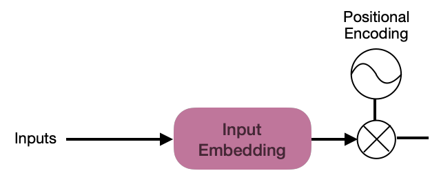
Starting at the beginning, the Transformer architecture begins with the Input Embedding sublayer, which converts the input sequence into vectors of dimension d_{model}=512.
🎓 The value of d_{model}=512 was set by the architecture designers to establish a constant dimension at the output of each sublayer of the model. The value of this dimension can be modified depending on the objectives.
A tokenizer transforms the input stream into tokens by normalizing the text to lowercase and truncating it into subparts; additionally, it will provide an integer vector representation (based on an existing vocabulary) that will be used for the embedding process. For example:
Input = "Roses are red and violets are blue"
Tokens = ["roses", "are", "red", "and", "violets", "are", "blue"]
Tokenized = [8271, 1029, 3674, 9273, 2384, 1029, 9873]
Next, the embedding sublayer is fed from the tokenized vector. For each word, this sublayer should produce a vector of size d_{model}=512. For example, for the words “red” and “blue,” which are colors, the word embedding vectors should be similar:
blue=[ 0.36138474, -0.16811648, -0.03733656, -0.58750702, -0.81279167,
       -0.86249844,  0.69673459, -0.79213212,  0.9278906 ,  0.42308278,
       -0.12308109,  0.2383174 ,  0.44863208,  0.98666162, -0.12830655,
       -0.56420363,  0.69459217,  0.72405279,  0.92023563, -0.84536481,
        0.86299045, -0.88166481, -0.9087216 ,  0.99420482, -0.73118714,
...
       -0.47495972, -0.94366021, -0.97624231, -0.9792538 ,  0.20736778,
        0.1248088 ,  0.6344501 , -0.54432975, -0.35632176, -0.6670839 ,
       -0.48141856, -0.3503394 , -0.94319604,  0.48421567, -0.12854877,
       -0.48260166, -0.845398  ,  0.67561689,  0.29778234,  0.03009221,
        0.25067641, -0.81864996, -0.51513235, -0.44608639, -0.65686229]
🎓 Cosine similarity can be used to check if two embedding vectors are similar. For more information on the theory: Scikit-Learn’s Cosine Similarity.
Embedding vectors provide a lot of information to the Transformer about how the words in a sequence are related. However, information is still needed to indicate the position of the words in a sequence, and the Positional Encoding process is used for this.
Positional Encoding (PE)
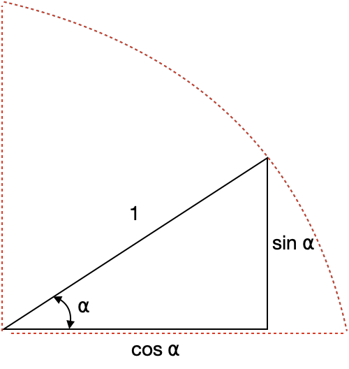
Each word in the initial sequence must have PE information, but the generation of this vector must be simple since the main focus of the Transformer is the attention mechanism.
The challenge in this task is to generate a vector of dimension d_{model}=512 to each output vector of the PE function. The architecture authors found a clever way to use a unit sphere to represent the PE with sine and cosine values.
🎓 With the idea of the unit sphere, the authors proposed sine and cosine functions that can generate different values of PE y for each dimension i of the 512 established in the word embedding vector.
PE_{(pos\:2i)}=sin \left (\frac{pos}{10000^{\frac{2i}{d_{model}}}} \right)(Plot sin in Google)
PE_{(pos\:2i+1)}=cos \left (\frac{pos}{10000^{\frac{2i}{d_{model}}}} \right) (Plot cos in Google)
The process will apply the sine function to even numbers i\: \in \left [ 0,\:255\right ] and the cosine function to odd numbers i\: \in \left [ 256,\:512\right ]. PE values are encoded within the unit sphere and allow a simple representation of the position of elements in the sequence.
The following example is a Python translation of the concept for Positional Encoding, evaluated for position 3:
import math

d_model = 512


def positional_encoding(position):
    pe = [None] * d_model

    for i in range(0, 512, 2):
        pe[i] = math.sin(position / (10000 ** ((2 * i) / d_model)))
        pe[i + 1] = math.cos(position / (10000 ** ((2 * i) / d_model)))

    return pe


print(positional_encoding(3))
For example, suppose we have the sentence “The sky is blue,” the positional encoding PE array will be:
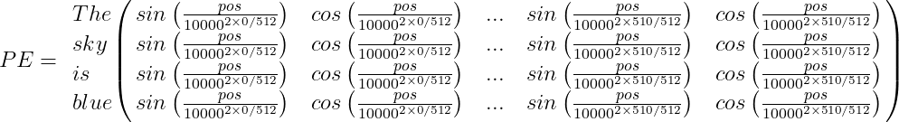
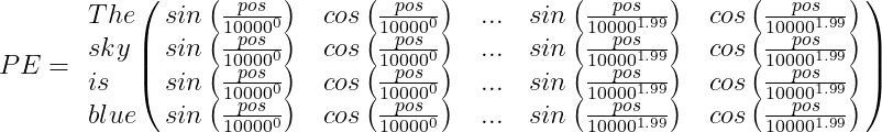
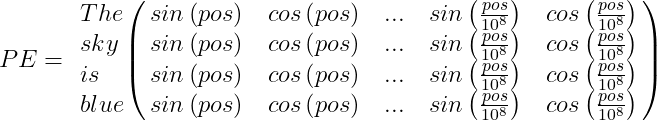
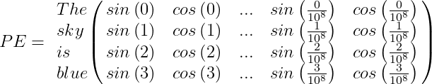
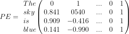
Finally, the word encoding vector should be added to the positional encoding vector, and the encoder/decoder block will be fed with the result:
Embedding_{output} = Embedding_{initial}+PE_{word\:position}
However, the word embedding values sometimes are too small and could be virtually disregarded. In this case, the solution is scaling the values by, for example, the PE mean.
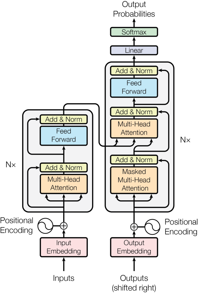
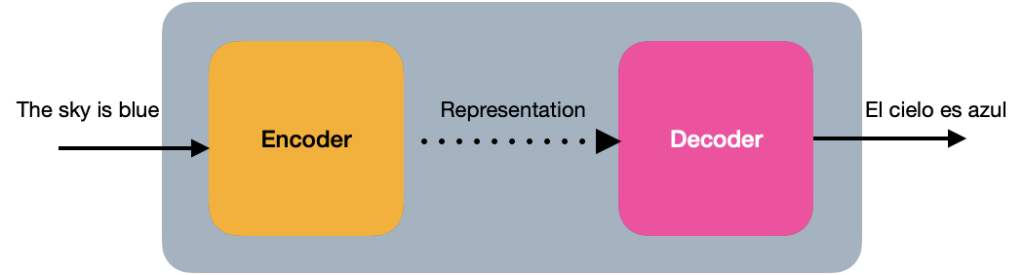
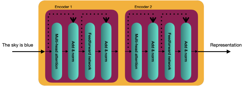
The encoder
In its simplest view, the Transformer is an encoder-decoder architecture, where the encoder learns the Positional Encoding representation of the input text and sends it to the decoder. The decoder receives what has been learned by the encoder and generates an output.
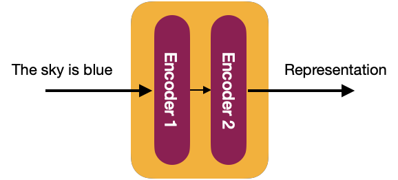
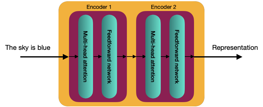
Internally, in more detail, the Transformer consists of a stack of N encoders, each sending its output to the next. The final encoder returns the representation of the input stream. For the explanation, from now on, we will use a value of N=2.
🎓 The original authors of the Transformer assigned the value of N=6 in “Attention is all you need”.
Each decoder block is composed of 2 sublayers:
- Multi-head attention
- Feedforward Network
Before starting to explain these two components, it is necessary to understand the self-attention mechanism.
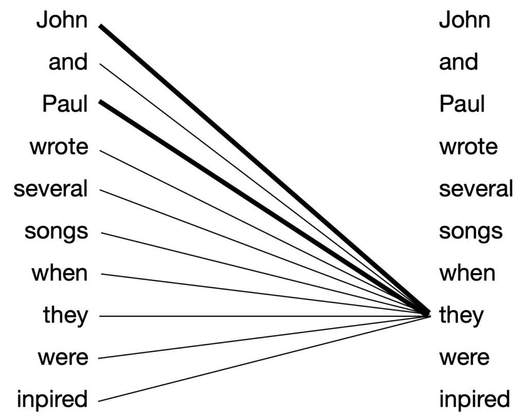
Self-attention Mecanism
Consider the following sentence:
John and Paul wrote several songs when they were inspired.
In this sentence, the self-attention mechanism computes the representation of each word, and the relationship with the other words in the sentence gives more information about the word. For example, the term “they” should be related to “John” and “Paul” and not to “songs.”
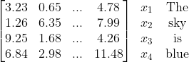
A more straightforward example of understanding how the self-attention mechanism works is the sentence “The sky is blue.” The encoders receive word embedding vectors of dimension d_{model}=512 of each word of the sentence, for example:
x_1=\begin{bmatrix} 3.23 & 0.65 & ... & 4.78 \end{bmatrix} ==> “The”
x_2=\begin{bmatrix} 1.26 & 6.35 & ... & 7.99 \end{bmatrix} ==> “sky”
x_3=\begin{bmatrix} 9.25 & 1.68 & ... & 4.26 \end{bmatrix} ==> “is”
x_4=\begin{bmatrix} 6.84 & 2.98 & ... & 11.48 \end{bmatrix} ==> “blue”
With these vectors we can assemble the embedding matrix X, with d=[4 \times 512]:
We will create three additional matrices from this matrix X that serves as the “self-attention mechanism.”:
- Q, query matrix
- K, key matrix
- V, value matrix
To create these arrays, we additionally need three new weight matrices. The dimension used in the original paper was d_k=64; therefore, the weight vectors would be of dimension d_{model} \times d_k\Rightarrow 512 \times 64, which are initialized with random values:
- W^Q, query weight matrix
- W^K, key weight matrix
- W^V, value weight matrix
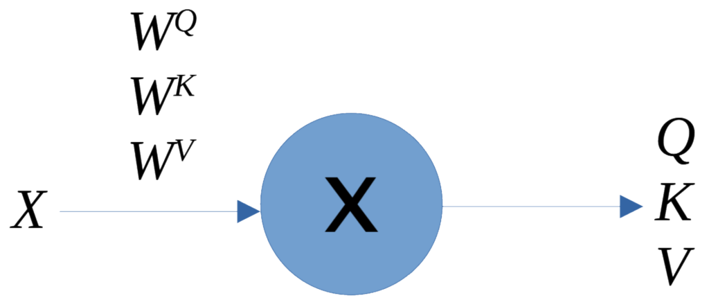
The weight matrices carry the optimal values learned during training, so each matrix Q, K, and V, is the product of the embedding matrix X with the corresponding weight matrix, which generates matrices 4 \times 64:
- Q = X \times W^Q
- K = X \times W^K
- V = X \times W^V
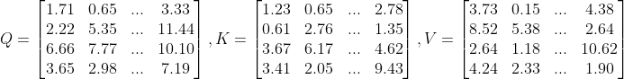
Each of the four rows in each matrix represents each word of the opening sentence, “The sky is blue.”
Self-attention Mechanism Process
1. Compute the dot product Q \cdot K^T
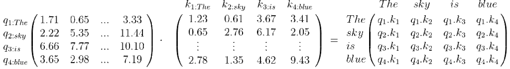
The elements of the resulting array indicate the relationship between the words. For example, q_1.k_1 is the relationship of the word “The” to itself and is a high value, but q_1.k_3 is the relationship between “The” and “is” and is a low value. The relationship between “sky” and “blue” (q_2.k_4) will have a slightly higher value because there is a relationship between the noun and the adjective. For example:
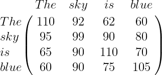
In this way, we can say that computing the dot product between the query matrix, Q, and the key matrix, K^T, essentially gives us the similarity value, which helps us understand how similar each word is in the sentence to all the other words.
2. Compute QK^T/\sqrt{d_k}. This action is useful to obtain stable gradients, where d_k=64 is the key vector dimension.
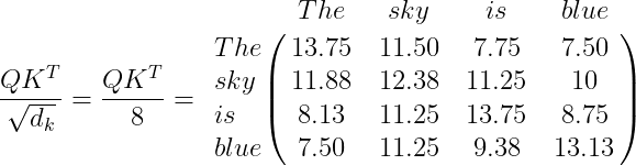
The values of the resulting matrix must be normalized, and if we use the function Softmax\left ( \frac{QK^T}{\sqrt d_k} \right ) (see Softmax), we can formalize the values in a range from 0 to 1.
import numpy as np


def softmax(x):
    max = np.max(x,axis=1,keepdims=True)
    e_x = np.exp(x - max)
    sum = np.sum(e_x,axis=1,keepdims=True)
    f_x = e_x / sum
    return f_x

V = np.array([[13.75, 11.50, 7.75, 7.50],
        [11.88, 12.38, 11.25, 10],
        [8.13, 11.25, 13.75, 8.75],
        [7.5, 11.25, 9.38, 13.13]])
softmax(V)
array([[0.90105641, 0.09497065, 0.0022335 , 0.00173945],
       [0.29994872, 0.49453184, 0.15975023, 0.04576921],
       [0.00331791, 0.07513861, 0.91537572, 0.00616775],
       [0.00304195, 0.12934693, 0.01993542, 0.8476757 ]])
The sum of the values in each row is equal to 1. With these values, we can understand how each word in the sentence relates to all the other words. This is called the score matrix.
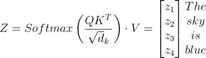
3. Next, we need to calculate the attention matrix Z:
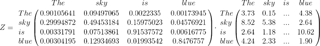
Z=\begin{bmatrix} 4.18336201 & 0.65278898 & ... & 4.22437426 \\ 5.94802206 & 3.00072113 & ... & 4.4028484 \\ 3.09529998 & 1.49925765 & ... & 9.9459073 \\ 4.76015677 & 2.69495094 & ... & 2.17709763 \end{bmatrix}
The attention matrix Z is a matrix of, for the example sentence, 4 rows, and 512 columns. Each row corresponds to the self-attention vector of the corresponding word.
The self-attention mechanism is called scaled dot product attention since we are computing the dot product between the vectors Q and K and scaling the values by (\sqrt {d_k}).
Multi-head attention mechanism
For the Transformer, we are going to compute multiple attention matrices. But why do we need multiple arrays? It helps us in idiomatic contexts where the meaning of a word is ambiguous, for example:
Tom was crying because he was blue.
A single attention mechanism would decide that Tom was crying because his color is blue, being dominated by the word “Tom.” And if most sentences in which “blue” implies that it is a color, by having only one “attention head,” the mechanism will correctly learn that it is a color. However, having “multiple attention heads,” one of those attention mechanisms is more likely to learn from the sentences in which it implies that “blue” is a mood, and by concatenating the results of the “multiple attention heads,” the attention matrix will be more accurate.
How do we compute multiple attention matrices? Suppose we are going to compute two attention matrices: Z_1 y Z_2.
To compute Z_1 first, we create the three matrices Q_1, K_1, and V_1, which implies multiplying the embedding matrix and the three weight matrices W_{1}^{Q}, W_{1}^{K}, and W_{1}^{V}. Now, the attention matrix is computed in the following way:
Z_1=Softmax\left ( \frac{Q_1K_{1}^{T}}{\sqrt{d_k}} \right ) \cdot V_1
In the same way for Z_2
Z_2=Softmax\left ( \frac{Q_2K_{2}^{T}}{\sqrt{d_k}} \right ) \cdot V_2
In this way, we can compute any number of attention matrices. Suppose we need eight attention matrices (the value in “Attention is all you need”). In that case, we can concatenate all the attention heads and multiply the result by a new weight matrix W_0 trained to represent the optimal values for the attention mechanism.
Multi-head \: attention=Concatenate\left ( Z_1, Z_2, Z_3, Z_4, Z_5, Z_6, Z_7, Z_8 \right ) \cdot W_0
Feedforward Network
The feedforward network consists of just two dense layers with ReLU activation. The same parameters are applied in the different places of the sentence, but it is other than the encoder blocks.
An additional component to connect the input and the encoder’s blocks is the add and norm component, which is a connection followed by layer normalization.
Layer normalization enables faster training by preventing the values in each layer from changing heavily.
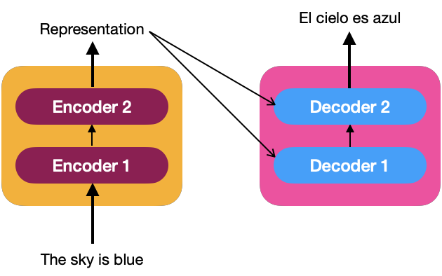
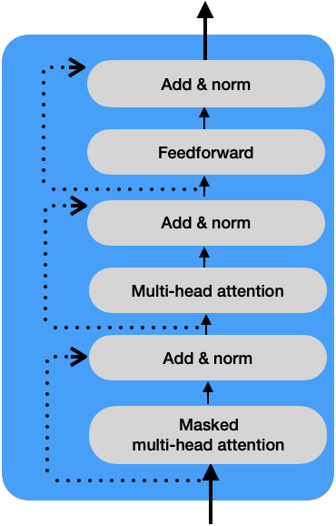
The decoder
In the same way as the encoder, we can have a stack of N decoders (for example, we assume that N=2). The representation of the sequence produced by the encoders is the input of all decoders; that is, a decoder receives two inputs, one from the previous decoder and the representation made by the encoder.
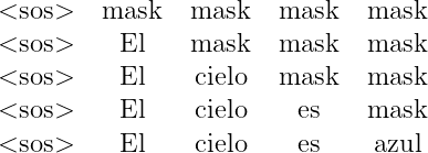
To understand how the decoder generates the target sentence, let’s look at the following image that describes the input to the decoder as a time series.
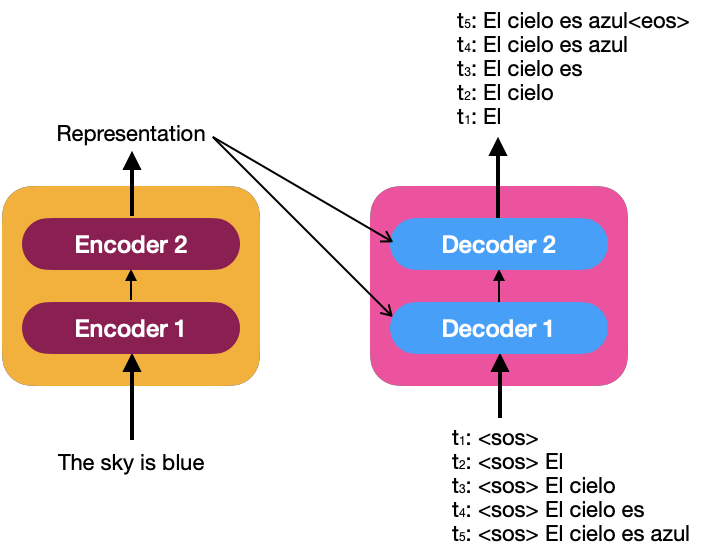
<eos>: End Of the Sentence
At each time step, the decoder matches the newly generated word to the input and predicts the following input. Once token <eos> is generated, the decoder has finished generating the target sentence.
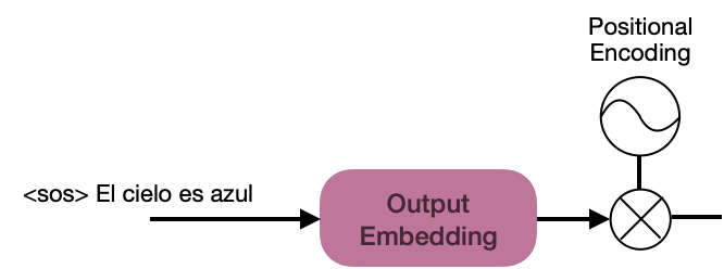
Like the input embedding for the encoders, the sentence “<sos> El cielo es azul” must be embedded to feed the decoders.
To understand how the decoder works, you must explore its components in the image below:
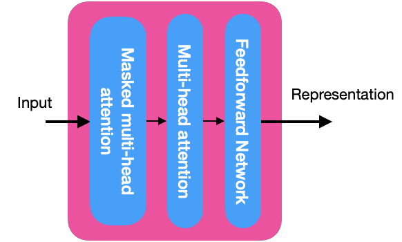
Masked multi-head attention
The masked multi-head attention is similar to the multi-head attention mechanism with a slight difference.
During a test, the decoder will generate words as long as there is a previous value; that is, for the input at “t2: <sos> El”, the model is trained only with the tokens <sos> and El, and the attention mechanism must match the words only up to the word El and not for the missing words in the sentence. The rest of the words in the sequence can be masked, which helps the attention mechanism to attend only to the words available during the tests.
We must compute the attention matrix Z the same way as we have been doing it, with the difference that the values corresponding to the masked word of the sentence receive a value of -\infty. For example:
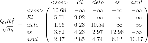
With this, we can get the final attention matrix as we did for the encoder, and this matrix will feed the next layer of multi-head attention.
Masked \; multihead \; attention=Concatenate\left ( Z_1, Z_2, Z_3, Z_4, Z_5, Z_6, Z_7, Z_8 \right ) \cdot W_0
Multi-head Attention
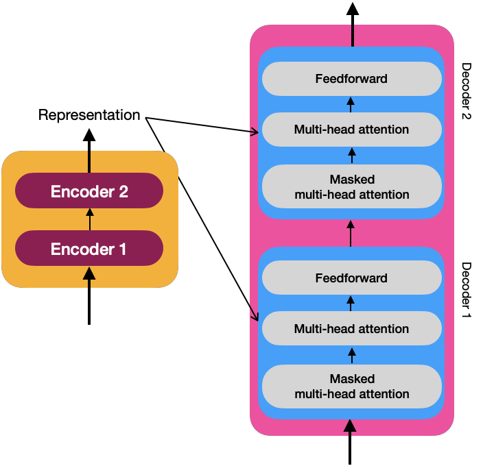
In the previous image, you can see the internal details of the decoders, and each multi-head attention layer receives the representation R of the output of the encoders and the masked multi-head attention M of the previous layer. Due to this layer’s interaction between the decoder and the encoder, it is also called encoder-decoder attention.
To calculate the attention mechanism, we obtain the query matrix Q using the matrix M; and the matrices K and V using the matrix R.
- Q_i = M \times W_i^Q
- K_i = R \times W_i^K
- V_i = R \times W_i^V
Q_i represents the target sentence obtained from M, and the matrices K and V contain the representation R obtained from the encoders.
Following is the procedure for obtaining the self-attention matrix:
Z_i=Softmax\left ( \frac{Q_iK_{i}^{T}}{\sqrt{d_k}} \right ) \cdot V_i
When computing the product Q_iK_{i}^{T}, we will observe that the result will contain a matrix that approximates the identity matrix, which helps us understand how similar Q (which represents the target sentence) is to the matrix K (representing the source sentence). For example:
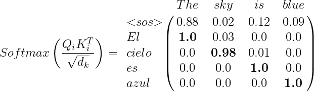
The attention matrix is obtained in the same way as in the previous sections:
Multihead \; attention=Concatenate\left ( Z_1, Z_2, Z_3, Z_4, Z_5, Z_6, Z_7, Z_8 \right ) \cdot W_0
Feedforward Network
This layer in the decoder works the same way as in the encoder. The add and norm component connects the input and output sublayers, as shown in the following picture:
Linear and Softmax Layer
The decoder learns the target sentence’s representation, which will be fed to the linear and softmax layers.
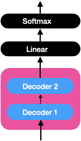
Linear Layer
This layer generates the logits with the size of the vocabulary. Assuming the vocabulary is:
Vocabulary=\left [ azul, cielo, El, es \right ]
Assuming that the input to the decoder is ” El,” the vector of logits generated by the decoder, for example, would be:
logits=\left [ 40, 51, 43, 38 \right ]
Softmax Layer
When we apply the Softmax function to the vector of logits above, we obtain a vector of probabilities, for example:
prob=\left [ 0.005, 0.973, 0.015, 0.007 \right ]
The vocabulary word with the highest probability value is “sky,” so this word is the decoder’s next prediction.
Transformer Training
The goal of model training is to minimize the loss function. For the Transformer, we have to minimize the difference between the predicted and actual probability distributions. The loss function that best suits this type of scenario is the “cross-entropy loss function,” and we use the Adam optimizer.
We apply dropout to each sublayer’s output and the sum of embeddings and positional encoding to prevent overfitting.
Conclusion
The concepts shown in this post are essential for understanding the internal workings of currently well-known models such as GPT-3, BERT, and other more modern ones such as PaLM. Understanding them will help us better appreciate and take advantage of the benefits of these Transformer models for NLP models in developing creative solutions like ChatGPT.
If you think this content is helpful, consider buying me a coffee. 😉☕️👉🏼