The purpose of this document is to present the linear classification algorithm SVM. The development of this concept has been based on previous ideas that have supported the development of SVM as an algorithm with good generalization capacity, based on an optimization criterion that minimizes complexity; with which we have achieved substantial improvements in terms of complexity and generalization with respect to similar classification algorithms.
The motivation to explore and show SVM in this document is to have an alternative algorithm that adapts to scenarios where other classification methods show weaknesses. We will explain the algorithm and show a comparative example to show its benefits.
Regarding the state of the art, there are currently several algorithms suitable for classification tasks:
- Linear Classifiers
- Decision Trees
- Random Forest
- Neural Networks
- Nearest Neighbor
Each algorithm has its applicability, its strengths and weaknesses. A weakness we have observed, for example, with decision trees is that they have a high classification error rate with few data and several classes, and that they are prone to over-fitting. We have also observed that linear classifiers are prone to have a high bias.
It is of great importance the visualization of the data and the way in which the classification algorithm behaves, and considering the results of Random Forest, even when they are acceptable, they are not easy to interpret visually: this is a very important lack because by observing the results of the classification process we can understand the behavior and make decisions.
Generally, Neural Networks are very powerful, but they are also more computationally demanding than other algorithms, which makes complicated implement them in, for example, Field-Programmable Gate Array chips (FPGA). Less powerful algorithms may be suitable for most scenarios and could be implemented without many problems in modern hardware only or mixed solutions.
Specifically, we mention Ridge Regression (RR) applied in classification because, comparing it with SVM, they share similar characteristics, but SVM simplifies and improves certain aspects.
One of these similarities, and where SVM makes a difference, is that SVM consists of the criterion based on Structural Risk Minimization, plus a linear loss function (Empirical Risk). This Structural Risk adds a regularization, which is a control of the learning machine’s complexity; criteria being used by both SVM and RR.
As we can see, RR shares the same structural risk; however, the loss function is based on a quadratic criterion; in this case, very high errors introduced by misclassified data can bias the result.
Ridge Regression

On the other hand, regularization in SVM is similar to RR, but we obtain a resolution for ω from an ordinary linear loss function:
SVM

This condition is an advantage for SVM, which makes it less sensitive to errors introduced by incorrectly classified outliers.
Approach
In a learning machine, Risk R(α) is the expectation of the error that we can get from evaluating distributed data x_n accordingly to a probability distribution function F(x). For each x_n we could have a label y_n, by this consideration we assume there is a conditional distribution between x and y: F(x|y).

Our objective is minimizing the error to make the learning machine useful, so we adjust this by minimizing the Risk. This Risk function must have a minimum in the point where a function of the error is minimized over all samples.

However, this concept of R(α) cannot be computed because F(x) and F(x|y) are unknown, so we need to compute an expectation based on the samples we have available, this is the Empirical Risk.

From this concept, we can see that we need to minimize the Empirical Risk, and the estimation function f(x,α) is what decides if data is correctly evaluated. However, having a machine with a very complex f(x,α) can make all results from testing data to be always correct, and this is not good because the Empirical Risk will tend to zero (over-fitting).
As we see, we have to limit the complexity of the machine, this minimization can be done by using the criteria to minimize the empirical risk: Structural Risk Minimization (SRM).
An important concept used to derive SVM is the Vapnik-Chervonenkis (VC) Dimension. As an example, we consider the 2-D space and 3 points. We have 3 possible positions for a classification hyperplane separating the points, which indicates 2 points are linearly independent.

What happens if we have 2 points? We can correctly classify them in any way, no matter how the points are shattered (over-fitting).

What happens if we have 4 points? We cannot classify them in all the possible ways.

As a conclusion, VC Dimension “h” is the maximum number of data points that can be shattered, and it gives us a measure of the complexity of linear functions. In a 2-D space, it is 3.
h=n+1
The VC Theorem says the following:
“Consider a set of m points in space Rn. Choose any one of the points as origin. Then the m points can be shattered by oriented hyperplanes if and only if the position vectors of the remaining points are linearly independent.”
As we see from the previous enunciate of VC Dimension, on the space R^2 with 4 points, we cannot always separate them by a hyperplane, because in the case(s) it fails, the remaining points are not linearly independent.

When we have 2 points in R^2, they will be always correctly classified, no matter how they are shattered, then the risk is always zero.
Clearly, if we have less points than dimensions n+1 we can always classify them correctly. This is not good because any classifier will make zero errors, causing over-fitting.
SVM consists on minimizing the empirical and structural risk (structural risk minimizes the complexity) in linear machines by explicitly limiting the VC Dimension of the hyperplane, but this is not real because data is linearly separable on it, and empirical risk is just zero. We need to define an empirical risk function that takes in account the samples that are INSIDE or ON the margin.
Consider a non-separable set of data D and slack variables ξ_n as:

ξ_n are zero for data outside the margin:

The idea consists on minimizing the empirical risk, which is the sum of all the slack variables:

SVM consists on minimizing the previous empirical risk plus the structural risk, which minimizes the complexity:

This condition applies to misclassified or inside the margin samples. If ξ_n<0, the sample is outside the margin and properly classified.
C is a tradeoff parameter that weights the importance of the empirical risk with the importance of the structural risk.
We start with the definition of the Karush-Kuhn-Tucker (KKT) Conditions:

We need to replace these conditions into the Lagrangian:

Let’s start with KKT (1):

Now, replace condition in term A:

And, replace condition in term CC:

Now, from KKT (4): μ_n ξ_n=0, we can see that D can be removed.
And from KKT (3): ∑_(n=1)^N▒〖α_n y_n=0〗, we can see that a term from the resultant CC can be removed.
Now we have the following:

Analyzing the latest term, we see that we can remove it.
- If sample is ON the margin: 0≤α_n≤C, and ξ_n=0
- If sample is INSIDE the margin: ξ_n>0, and α_n=C
Finally, we have the result:

In matrix notation:

This equation must be optimized with respect to the dual variables. Here X^T X is a Gram matrix of dot products: K_(i,j)=x_i^T x_j
The dual can be written as follows:

Some properties of Support Vectors are the following:
- Support Vectors ON margin have a relationship with the VC Dimension, as for in R2 we ALWAYS have 3 support vectors ON margin.
- Support Vector are INSIDE or ON the margin
- For Support Vectors ON margin, 0 < alpha< C
- For Support Vectors INSIDE the margin alpha = C
When we have an outlier away from the margin and classification hyperplane, we know that .
SVM behavior remain stable and throwing good results with small and mid-size data, but the most important problem on SVM is that the term K that we mentioned before can be huge if we have a lot of data for training.
Experiment
In order to demonstrate SVM applied in data classification, we have built an experiment that can be executed on Matlab, previous installation of the public library LIBSVM, which implements the SVM algorithm. The complete code for the experiment, and LIBSVM’s documentation can be found on references.
For this experiment we have created a data set by generating 40 random data points sparse around 4 centroids, and classifying 20 of them as 1, and the other 20 as -1.
We start defining the initial data and, with help of LIBSVM, we train the model for SVM classification. With the initial data and trained model, we obtain results similar to the following:
optimization finished, #iter = 162
nu = 0.171989
obj = -617.860697, rho = -0.466784
nSV = 8, nBSV = 5
Total nSV = 8
Accuracy = 95% (38/40) (classification)
K>> model

model =
    struct with fields:

        Parameters: [5×1 double]
            nr_class: 2
             totalSV: 8
                 rho: -0.4668
               Label: [2×1 double]
          sv_indices: [8×1 double]
               ProbA: []
               ProbB: []
                 nSV: [2×1 double]
             sv_coef: [8×1 double]
                 SVs: [8×2 double]
Additionally, the model has the following information from α:
>> alpha

100.0000
43.9775
100.0000
100.0000
-100.0000
-100.0000
-93.3429
-50.6346
The accuracy of the model is 92.5%, and comparing with the α array, we can see that we have only 5 misclassified or in margin points (±100, as C was declared 100 when we used LIBSVM, so α = C), and 3 points ON the margin.
We have compared manually calculated results with the predicted results:

- Inside Margin (yellow)
- On Margin (green)
- Misclassified (red)
As we can see, the results are similar between manually evaluating the equation, and the results from LIBSVM iterations (162 iter); except for 1 value incorrectly evaluated as “well classified”, when it is misclassified, as we will see in the next plot with data points and the following equations:
- ω^T x+b=1 (blue)
- ω^T x+b=0 (green)
- ω^T x+b=-1 (red)

From this plot we see that data points are being classified by the AVM model we built with LIBSVM, and we can mention the following conclusions:
- After running the script several times, we can see the we ALWAYS have 3 support vectors for this 2D space, and we see the VC Theorem working on SVM.

- As we saw in the comparison between predicted and Y, there are 2 misclassified points

- As we saw in alpha values, we have 3 points ON the margin, and 5 points misclassified or INSIDE margin.

We also tried with data points less sparse around centroids, and we see that the machine always correctly classifies all data points, as they are clearly separated and machine can interpret them correctly, as we can see in Figure 5.
In the same way, we tried with data points widely sparse around centroids, and we can see that data are approaching to the other centroids (or getting away). As result, we can see it is harder for the machine to correctly classify data points, as depicted in Figure 6.


Conclusions
SVM is an algorithm based on SRM, which offers the advantage of a large generalization capacity.
The results of an experiment have been presented using data generated automatically by software, through which we can see the features of the algorithm, and its behavior with low, medium, and highly scattered data, and we can understand its robustness.
One of the best benefits we obtain from SVM is that when we have an outlier away from the margin and classification hyperplane, we know that α=C. It is important because its maximum contribution on error is C, it will not affect the behavior of the machine.
Comparing with the other classification algorithms, it is clear that now we have an option less sensitive to misclassified outliers. It is visually understandable, so it makes suitable to graphically observe the classifier’s behavior. It is also simple enough to derive mixed versions on FPGA, where we can codesign part of the algorithm with hardware and software (C code).
SVM behavior remain stable and throwing good results with small and mid-size data; however, the most important problem on SVM is that the term K that we mentioned before can be huge if we have a lot of data for training.
As we understand now, SVM classification gives us good results, and it fits in several researching scenarios as a good alternative to other algorithms. For future works, we need to apply these concepts for non-linear machines.
References
- Types of classification algorithms in Machine Learning, By. Mandeep Sidana, Technology Consultant, Sifium Technologies. Available: https://medium.com/@sifium/machine-learning-types-of-classification-9497bd4f2e14
- Classification Model Pros and Cons, By. Chris Tufts. Available: https://github.com/ctufts/Cheat_Sheets/wiki/Classification-Model-Pros-and-Cons
- LIBSVM, Software and Documentation, By. Chih-Chung Chang and Chih-Jen Lin. Available: https://www.csie.ntu.edu.tw/~cjlin/libsvm/

