Update 09.2022
This entry has been updated to TensorFlow v2.10.0 and PyTorch 1.12.1
Table of Contents
What is an activation function?
An activation function is a function that is applied to a neuron in a neural network to help it learn complex patterns of data, deciding what should be transmitted to the next neuron in the network.
A perceptron is a neural network unit that inputs the data to be learned into a neuron and processes it according to its activation function.
The perceptron is a simple algorithm that, given an input vector x of m values(x_1, x_2, ..., x_m), outputs a 1 or a 0 (step function), and its function is defined as follows:


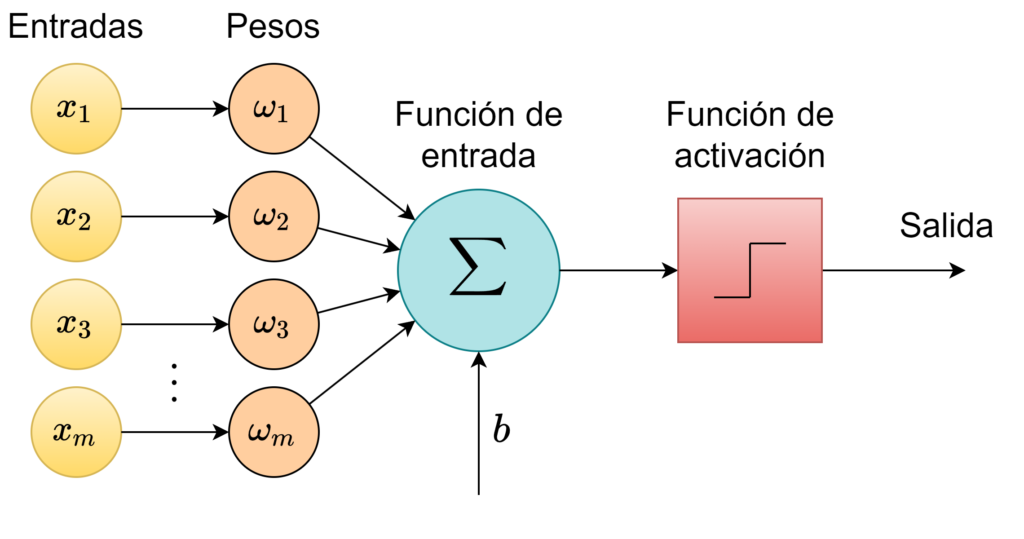
Here, ω is a vector of weights, ωx is the dot product, and b is the bias. This equation reassembles the equation of the line. If x is on this line, the answer is positive; otherwise, it is negative. However, ideally, we will pass in training data and allow the computer to adjust the weight and bias so that the errors produced by this neuron are minimized. The learning process should recognize small changes that progressively teach our neurons to classify information as we want.
The following image is a step function where if x>0, the output is 1, and if x<0, the result is 0. It is useless as an activation function since we do not have “small changes,” but significant changes, and the neuron cannot learn in this way since ω and b will not converge to the optimal values to minimize errors.
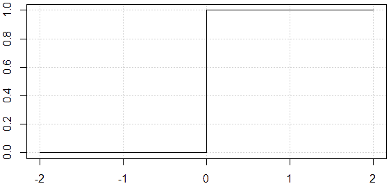
The tangent of the activation function indicates whether the neuron is learning; From the previous image, we deduce that the tangent at x=0 is \infty. This value is unreal because, in real life, we learn everything step by step. For a neuron to learn, we need something that changes progressively from 0 to 1, that is, a continuous (and differentiable) function.
When we started using neural networks, we used activation functions as an essential part of a neuron. This activation function will allow us to adjust weights and biases.
The derivative of the activation function feeds the backpropagation during learning. For this reason, the function and its derivative must have a low computational cost.
Activation Functions
Currently, there are several types of activation functions that are used in various scenarios. Below is a short explanation of the activation functions available in the tf.keras.activations module from the TensorFlow v2.10.0 distribution and torch.nn from PyTorch 1.12.1.
Sigmoid
\sigma \left ( x \right )=\frac{1}{1+e^{-x}}
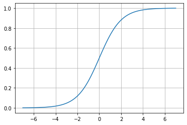
Mathematically, this function is continuous. As we can see, in the sigmoid, the changes are gradual, and we can have values other than 0 or 1.
![]() Example:
Example:
import tensorflow as tf
import matplotlib.pyplot as plt

X = tf.linspace(-7., 7., 100)
y = tf.keras.activations.sigmoid(X)
plt.plot(X,y)
plt.grid()
![]() Example:
Example:
import torch
import matplotlib.pyplot as plt

X = torch.linspace(-7., 7., steps=100)
y = torch.nn.Sigmoid()(X)
plt.plot(X,y)
plt.grid()
See it at Google Colab here: Activation Functions
The sigmoid function is the most common activation function; however, it is not used frequently due to the tendency to drive the backpropagation terms to zero during training.
ReLU (Rectified Linear Unit)
f(x)=max(0,x)
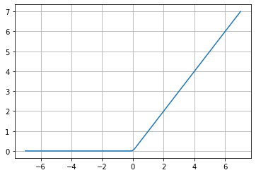
This function has become very popular as it generates excellent experimental results. The most significant advantage of ReLU is that this function speeds up the Stochastic Gradient Descent (SGD) convergence, which indicates how fast the neuron is learning, compared to the Sigmoid and Hyperbolic Tangent functions.
This strength is, in turn, its greatest weakness since this “learning speed” can cause the weights \omega of the neuron to be updated and oscillate from the optimal values and not be activated at any point. For example, if the learning rate is too high, half of the neurons may be “dead,” but if an appropriate value is set, the neurons will learn, but it will be slower than expected.
![]() Example:
Example:
import tensorflow as tf
import matplotlib.pyplot as plt

X = tf.linspace(-7., 7., 100)
y = tf.keras.activations.relu(X)
plt.plot(X,y)
plt.grid()
![]() Example:
Example:
import torch
import matplotlib.pyplot as plt

X = torch.linspace(-7., 7., steps=100)
y = torch.nn.ReLU()(X)
plt.plot(X,y)
plt.grid()
See it at Google Colab here: Activation Functions
ReLU6
f(x)= min(max(0,x), 6)
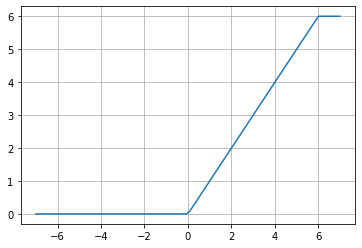
This function has historically remained in the tf.nn module, inherited from TensorFlow 1. It was introduced in the paper “Convolutional Deep Belief Networks on CIFAR-10” (page 2), with the advantage, compared to the simple ReLU, that it is computationally faster and doesn’t suffer from “exploding” values. As we can infer from the paper that introduced it, it has been used in Convolutional (CNN) and Recurrent (RNN) neural networks.
![]() Example:
Example:
import tensorflow as tf
import matplotlib.pyplot as plt

X = tf.linspace(-7., 7., 100)
y = tf.nn.relu6(X)
plt.plot(X,y)
plt.grid()
![]() Example:
Example:
import torch
import matplotlib.pyplot as plt

X = torch.linspace(-7., 7., steps=100)
y = torch.nn.ReLU6()(X)
plt.plot(X,y)
plt.grid()
See it at Google Colab here: Activation Functions
Hyperbolic Tangent
f(x)= tanh(x)
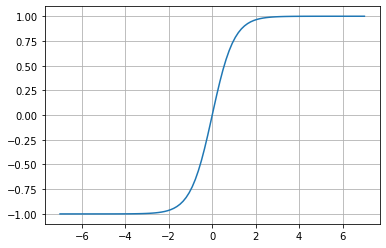
This function is similar to the sigmoid, but instead of having a range between 0 and 1, it ranges from -1 to 1. Sadly, it has the same vanishing problem as the sigmoid.
![]() Example:
Example:
import tensorflow as tf
import matplotlib.pyplot as plt

X = tf.linspace(-7., 7., 100)
y = tf.keras.activations.tanh(X)
plt.plot(X,y)
plt.grid()
![]() Example:
Example:
import torch
import matplotlib.pyplot as plt

X = torch.linspace(-7., 7., steps=100)
y = torch.nn.Tanh()(X)
plt.plot(X,y)
plt.grid()
See it at Google Colab here: Activation Functions
ELU (Exponential Linear Unit)
Given a value of \alpha>0
f(x)=x\;\;if\;\;x\geq 0
f(x)=\alpha (e^{x}-1)\;\;if\;\;x<0
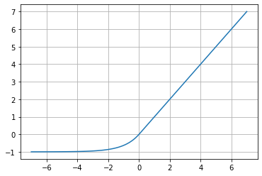
According to the paper “Fast and Accurate Deep Network Learning by Exponential Linear Units (ELUs)“, this function tends to converge to zero faster and produces more accurate results. Its behavior is similar to ReLU, but for negative values where it exponentially tends to -\alpha.
It’s a commonly used function on CNN, as their research paper indicates.
![]() Example:
Example:
import tensorflow as tf
import matplotlib.pyplot as plt

X = tf.linspace(-7., 7., 100)
y = tf.keras.activations.elu(X, alpha=1.0)
plt.plot(X,y)
plt.grid()
![]() Example:
Example:
import torch
import matplotlib.pyplot as plt

X = torch.linspace(-7., 7., steps=100)
y = torch.nn.ELU()(X)
plt.plot(X,y)
plt.grid()
See it at Google Colab here: Activation Functions
Softmax
Given a vector of values x, and a number of classes K of a multi-class classifier:

Softmax converts a vector of values to a probability distribution of sum 1; as we can see, its use differs from the rest of the activation functions in that this function is used as the final layer in classifiers based on neural networks.
This function is used in classifiers and reinforcement learning to convert values into performance probabilities. As Wikipedia (ES) indicates:
It correlates the expected reward for performing a specific action with the probability of choosing it. This way, the actions with the highest expected reward are selected with the most significant probability.
Wikipedia: Función Softmax
![]() Example:
Example:
import tensorflow as tf

inputs = tf.random.normal(shape=(32, 10))
outputs = tf.keras.activations.softmax(inputs)
tf.reduce_sum(outputs[0, :])  # Each sample in the batch now sums to 1
![]() Example:
Example:
import torch

inputs = torch.randn(32, 10)
outputs = torch.nn.Softmax(dim=1)(inputs)
torch.sum(outputs[0, :])  # Each sample in the batch now sums to 1
See it at Google Colab here: Activation Functions
Softplus
f(x)=ln(1+e^{x})
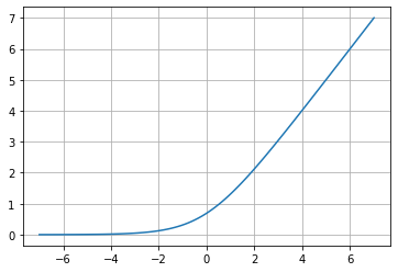
Softplus is an alternative to traditional functions, such as Sigmoid or Hyperbolic Tangent, because it is differentiable (essential for the backpropagation function). The amazing thing with the derivative of this function is that it is the Sigmoid function!
\frac{\partial y}{\partial x}=\left ( ln(1+e^x) \right )'=\left ( \frac{1}{1+e^x} \right )\left ( 1+e^x \right )'
\frac{\partial y}{\partial x}=\left ( \frac{1}{1+e^x} \right )\cdot e^x=\frac{e^x}{1+e^x}=\frac{e^{x}}{e^{x}\left ( e^{-x}+1 \right )}
\therefore\;\; \frac{\partial y}{\partial x}=\frac{1}{1+e^{-x}}
Interestingly, it allows us to understand more clearly how the backpropagation process will behave.
![]() Example:
Example:
import tensorflow as tf
import matplotlib.pyplot as plt

X = tf.linspace(-7., 7., 100)
y = tf.keras.activations.softplus(X)
plt.plot(X,y)
plt.grid()
![]() Example:
Example:
import torch
import matplotlib.pyplot as plt

X = torch.linspace(-7., 7., steps=100)
y = torch.nn.Softplus()(X)
plt.plot(X,y)
plt.grid()
See it at Google Colab here: Activation Functions
Softsign
f(x)=\frac{x}{\left ( 1+\left | x \right | \right )}
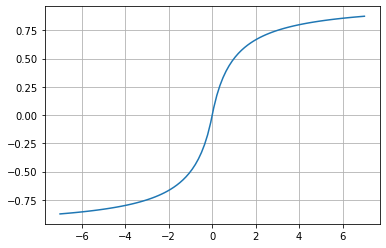
Given the shape of the graph, we can see that it is an alternative to Hyperbolic Tangent, but it has not been as widely adopted. However, considering that the activation function is state-of-the-art, it could be the function that best fits specific neural network models.
![]() Example:
Example:
import tensorflow as tf
import matplotlib.pyplot as plt

X = tf.linspace(-7., 7., 100)
y = tf.keras.activations.softsign(X)
plt.plot(X,y)
plt.grid()
![]() Example:
Example:
import torch
import matplotlib.pyplot as plt

X = torch.linspace(-7., 7., steps=100)
y = torch.nn.Softsign()(X)
plt.plot(X,y)
plt.grid()
See it at Google Colab here: Activation Functions
Swish
f(x)=\frac{x}{1+e^{-x}}
f(x)=x\cdot Sigmoid(x)
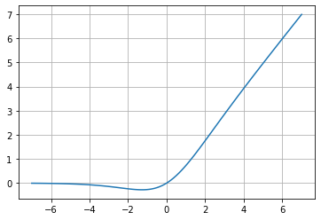
This activation function is relatively new (2017) and outperforms ReLU for deeper CNN networks. The equation that defines this function describes a Sigmoid(x), but it doesn’t have the gradient vanishing problem. The x factor makes this function important again.
Regarding its comparison with ReLU, ReLU had the problem of outputting 0 for negative values added to backpropagation; Swish partially handles this problem. However, the computational cost of Swish is higher. It is an issue you should evaluate for your decision since this cost carried over to the backpropagation process will increase.
![]() Example:
Example:
import tensorflow as tf
import matplotlib.pyplot as plt

X = tf.linspace(-7., 7., 100)
y = tf.keras.activations.swish(X)
plt.plot(X,y)
plt.grid()
![]() Example:
Example:
import torch
import matplotlib.pyplot as plt

# It's interesting that PyTorch doesn't have a built-in swish function
X = torch.linspace(-7., 7., steps=100)
y = X * torch.nn.Sigmoid()(X)
plt.plot(X,y)
plt.grid()
See it at Google Colab here: Activation Functions
Sinc
f(x)=\frac{sin(x)}{x}\;\;if\;\;x\neq 0
f(x)=1\;\;if\;\;x=0
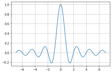
Sinc is an unusual activation function since it rises and falls in contrast to the other functions. However, the function saturates, and its output converges to zero for large positive and negative input values.
The function has an exception at x=0 since evaluating that value at f(x)=\frac{sin(x)}{x} would result in a divide-by-0 indetermination.
Periodic functions like Sinc are not popular in neural networks as activation functions. But even when sinc is periodic, it will saturate when the input value increases positively or negatively, just like other functions such as the Sigmoid or the Hyperbolic Tangent, which makes this function an interesting alternative as an activation function in neural networks.
![]() Example:
Example:
import tensorflow as tf
import matplotlib.pyplot as plt

X = tf.linspace(-7., 7., 100)
y = tf.experimental.numpy.sinc(X)
plt.plot(X,y)
plt.grid()
![]() Example:
Example:
import torch
import matplotlib.pyplot as plt

X = torch.linspace(-7., 7., steps=100)
y = torch.special.sinc(X)
plt.plot(X,y)
plt.grid()
See it at Google Colab here: Activation Functions
Leaky ReLU
Given a value of \alpha>0
f(x)=x\;\;if\;\;x\geq 0
f(x)=\alpha x\;\;if\;\;x<0
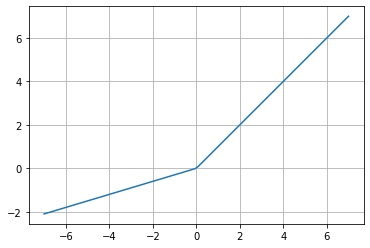
ReLU is a very popular activation function in CNN since for positive values; it does not saturate and stop learning; however, a weakness of the ReLU is that for negative values, it tends to saturate, and Leaky ReLU (LReLU) corrects this problem.
TensorFlow sets a default value for the constant \alpha=0.3, although some sources mention a value of 0.01. Roughly speaking, \alpha sets the slope of the equation for negative values, and LReLU improves the convergence performance.
![]() Example:
Example:
import tensorflow as tf
import matplotlib.pyplot as plt

X = tf.linspace(-7., 7., 100)
leakyReLU = tf.keras.layers.LeakyReLU(alpha=0.3)
y = leakyReLU(X)
plt.plot(X,y)
plt.grid()
![]() Example:
Example:
import torch
import matplotlib.pyplot as plt

X = torch.linspace(-7., 7., steps=100)
y = torch.nn.LeakyReLU(0.3)(X)
plt.plot(X,y)
plt.grid()
See it at Google Colab here: Activation Functions
Mish
f(x)=x\cdot tanh(softplus(x))
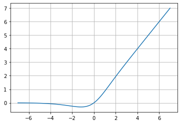
Due to its form, this function is very similar to Swish, defined as “a self-regularized non-monotonic activation function,” according to its research paper (2020). The innovative part of Mish is given by the intuitive understanding of the behavior of the derivative to understand how it helps to regularize the optimization of neural networks.
\frac{\partial y}{\partial x}=(x\cdot tanh(softplus(x)))'=(x\cdot tanh(1+e^{x}))'
\frac{\partial y}{\partial x}=\frac{e^{x}\omega }{\delta ^{2}}
Where:
\omega =4(x+1)+4e^{2x}+e^{3x}+e^{x}(4x+6)
\delta =2e^{x}+e^{2x}+2
These functions are easier to graph and better understand how the backpropagation process will behave.
![]() Example:
Example:
! pip install tensorflow-addons
import tensorflow as tf
import tensorflow_addons as tfa
import matplotlib.pyplot as plt

X = tf.linspace(-7., 7., 100)
y = tfa.activations.mish(X)
plt.plot(X,y)
plt.grid()
![]() Example:
Example:
import torch
import matplotlib.pyplot as plt

X = torch.linspace(-7., 7., steps=100)
y = torch.nn.Mish()(X)
plt.plot(X,y)
plt.grid()
See it at Google Colab here: Activation Functions
GELU (Gaussian Error Linear Unit)
f(x)=xP(X\leq x)=x\;\Phi (x)=x\cdot \frac{1}{2}\left [ 1+erf(\frac{x}{\sqrt{2}}) \right ]
f(x)\approx 0.5x\left ( 1+tanh\left [ \frac{\sqrt{2}}{\pi}\left ( x+0.044715x^{3} \right ) \right ] \right )
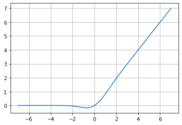
This function aims to merge the functionality of a Linear Unit (ReLU, ELU) with the Dropout regularization function through a stochastic multiplication of the input vector by 0 or by 1 and obtain the activation function in a deterministic way.
GELU, as determined in its research paper, is determined by a Gaussian distribution function which eliminates the negative vanishing problem that ReLU has, improving its performance for tasks such as computer vision, NLP, and speech processing.
![]() Example:
Example:
import tensorflow as tf
import matplotlib.pyplot as plt

X = tf.linspace(-7., 7., 100)
y = tf.keras.activations.gelu(X)
plt.plot(X,y)
plt.grid()
![]() Example:
Example:
import torch
import matplotlib.pyplot as plt

X = torch.linspace(-7., 7., steps=100)
y = torch.nn.GELU()(X)
plt.plot(X,y)
plt.grid()
See it at Google Colab here: Activation Functions
SELU (Scaled Exponential Linear Unit)
f(x)=\lambda x\;\;if\;\;x\geq 0
f(x)=\lambda \alpha (e^{x}-1)\;\;if\;\;x<0
Donde \alpha \approx 1.6733 y \lambda \approx 1.0507
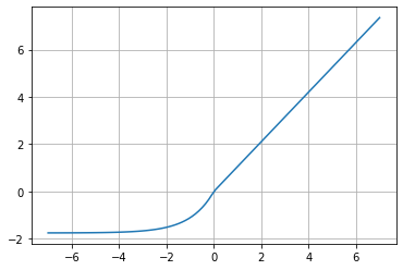
SELU is an activation function that induces self-normalizing properties that converges to zero mean and unit variance. Unlike ReLU, it can reach values below 0, which allows the neural network to have an output of mean 0, and this feature helps the model to converge more quickly towards the solution.
![]() Example:
Example:
import tensorflow as tf
import matplotlib.pyplot as plt

X = tf.linspace(-7., 7., 100)
y = tf.keras.activations.selu(X)
plt.plot(X,y)
plt.grid()
![]() Example:
Example:
import torch
import matplotlib.pyplot as plt

X = torch.linspace(-7., 7., steps=100)
y = torch.nn.SELU()(X)
plt.plot(X,y)
plt.grid()
See it at Google Colab here: Activation Functions
