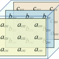
Matrices are the basic elements we use to interchange data through computational graphs. In general terms, a tensor can de defined as a matrix, so you can refer to Declaring tensors in TensorFlow in order to see the options you have to create matrices.
Let’s define the matrices we are going to use in the examples:
import tensorflow as tf
import numpy as np

sess = tf.Session()

identity_matrix = tf.diag([1., 1., 1., 1., 1.])
mat_A = tf.truncated_normal([5, 2], dtype=tf.float32)
mat_B = tf.constant([[1., 2.], [3., 4.], [5., 6.], [7., 8.], [9., 10.]])
mat_C = tf.random_normal([5, ], mean=0, stddev=1.0)
mat_D = tf.convert_to_tensor(np.array([[1.2, 2.3, 3.4], [4.5, 5.6, 6.7], [7.8, 8.9, 9.10]]))
Matrix Operations
Addition and substraction are simple operations that can be performed by ‘+’ and ‘-‘ operators, or by tf.add() or tf.subtract().
# A + B
>>> print(sess.run(mat_A + mat_B))
>>> print(sess.run(tf.add(mat_A, mat_B)))
 [[ 0.58516705 2.84226775]
 [ 2.3062849 4.91305351]
 [ 5.88148737 4.88284636]
 [ 6.40551376 6.56219101]
 [ 9.73429203 9.89524364]]
# B - B
>>> print(sess.run(mat_B - mat_B))
>>> print(sess.run(tf.subtract(mat_B, mat_B)))
[[ 0. 0.]
[ 0. 0.]
[ 0. 0.]
[ 0. 0.]
[ 0. 0.]]Matrices multiplication must follow the following rule:

If this rule is accomplished, then we can perform multiplication.
tf.matmul() performs this operation; as an option, previously we can transpose or adjointe (conjugate and transpose), and optionally we can mark any matrix as sparsed. For example:
# B * Identity
>>> print(sess.run(tf.matmul(mat_B, identity_matrix, transpose_a=True, transpose_b=False)))
 [[ 1. 3. 5. 7. 9.]
 [ 2. 4. 6. 8. 10.]]
Other operations
# Transposed C
>>> print(sess.run(tf.transpose(mat_C)))
 [ 0.62711298 1.33686149 0.5819205 -0.85320765 0.59543872]
# Matrix Determinant D
>>> print(sess.run(tf.matrix_determinant(mat_D)))
3.267# Matrix Inverse D
>>> print(sess.run(tf.matrix_inverse(mat_D)))
[[-2.65381084 2.85583104 -1.11111111]
[ 3.46189164 -4.77502296 2.22222222]
[-1.11111111 2.22222222 -1.11111111]]# Cholesky decomposition
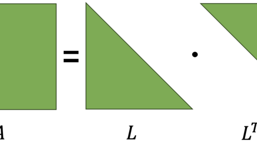
>>> print(sess.run(tf.cholesky(identity_matrix)))
[[ 1. 0. 0. 0. 0.]
[ 0. 1. 0. 0. 0.]
[ 0. 0. 1. 0. 0.]
[ 0. 0. 0. 1. 0.]
[ 0. 0. 0. 0. 1.]]# Eigen decomposition
>>> print(sess.run(tf.self_adjoint_eig(mat_D)))
(array([ -3.77338787, -0.85092622, 20.52431408]), array([[-0.76408782, -0.4903048 , 0.41925053],
[-0.21176465, 0.8045062 , 0.55491037],
[ 0.60936487, -0.33521781, 0.71854261]]))Element-wise Operations
# A * B (Element-wise)
>>> print(sess.run(tf.multiply(mat_A, mat_B)))
# A % B (Element-wise)
>>> print(sess.run(tf.div([2, 2], [5, 4])))
[0 0]# A / B (Element-wise)
>>> print(sess.run(tf.truediv([2, 2], [5, 4])))
[ 0.4 0.5]# A / B Floor-approximation (Element-wise)
>>> print(sess.run(tf.floordiv([8, 8], [5, 4])))
[1 2]# A/B Remainder (Element-wise)
>>> print(sess.run(tf.mod([8, 8], [5, 4])))
[3 0]Cross-product
>>> print(sess.run(tf.cross([1, -1, 2], [5, 1, 3])))
 array([-5, 7, 6], dtype=int32)
We’ve completed all theoretical prerequisites for TensorFlow. Once we understand matrices, variables and placeholders, we can continue with Core TensorFlow. See you next time!
